text causality December 9, 2015 In [1]: # HIDDEN from datascience - PDF document

text causality December 9, 2015 In [1]: # HIDDEN from datascience import * %matplotlib inline import matplotlib.pyplot as plots plots.style.use(’fivethirtyeight’) import pylab as pl import math from scipy import stats 0.1 Difference and Causality In the previous example, we asked whether the amount of radiation a patient received affected his/her 15- month score. Radiation and the 15-month score are distinct physical quantities, measured in different units. The scatter plot and regression are tools that help us measure the relation between such variables. However, if the variables are “like” quantities – that is, measured in the same units, such as the baseline score and 15-month score – then it might be possible to use simpler methods. In the following examples, we will try to see if we can identify a difference between two groups of “like” measurements; if there is a difference, we will see if we can identify the cause. How we go about doing this, and whether we succeed, will depend very much on the details of the randomization involved in the sampling. Example 1. Is there a difference between baseline scores and 15-month scores? If so, why? The first question we will address is whether there is a difference between the scores of the Hodgkin’s disease patients before and after treatment. In order to make an inference about this based on the data, we first note that the basline and 15-month scores are paired by patient – that is, there is one (baseline, 15-month) pair of scores for each patient. The interesting question is not whether the baseline and 15-month scores differ overall on average; it is whether there is a change in score per patient. 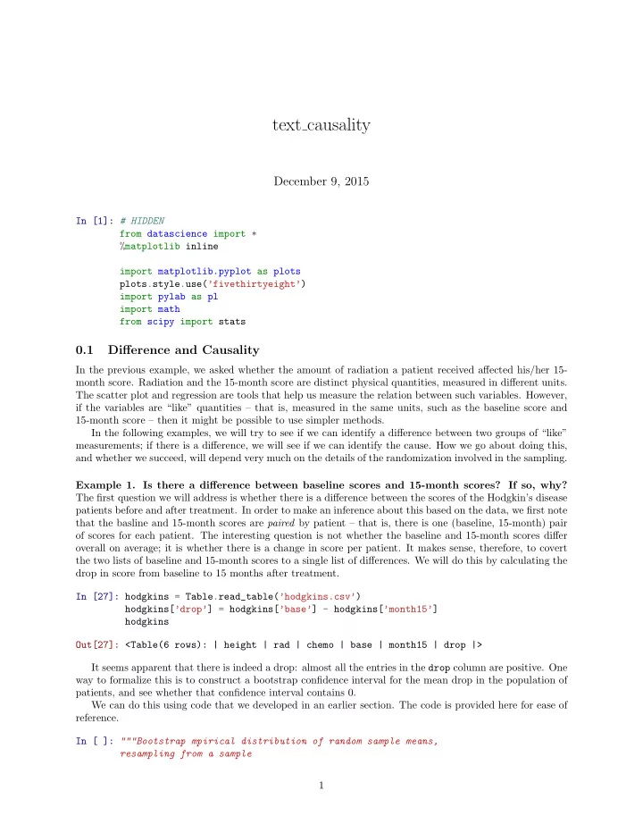It makes sense, therefore, to covert the two lists of baseline and 15-month scores to a single list of differences. We will do this by calculating the drop in score from baseline to 15 months after treatment. In [27]: hodgkins = Table.read_table(’hodgkins.csv’) hodgkins[’drop’] = hodgkins[’base’] - hodgkins[’month15’] hodgkins Out[27]: <Table(6 rows): | height | rad | chemo | base | month15 | drop |> It seems apparent that there is indeed a drop: almost all the entries in the drop column are positive. One way to formalize this is to construct a bootstrap confidence interval for the mean drop in the population of patients, and see whether that confidence interval contains 0. We can do this using code that we developed in an earlier section. The code is provided here for ease of reference. In [ ]: """Bootstrap mpirical distribution of random sample means, resampling from a sample 1

Arguments: table of original sample data, column label, number of repetitions""" def bootstrap_mean(samp_table, column_label, repetitions): # Set up an empty table to collect all the replicated medians means = [] # Run the bootstrap and place all the medians in the table for i in range(repetitions): resample = samp_table.select(column_label).sample(with_replacement=True) m = np.mean(resample[column_label]) means.append(m) # Display results means = Table([means], [’means’]) means.hist(bins=20,normed=True) plots.xlabel(’resampled means’) print("Original sample mean:", np.mean(samp_table[column_label])) print("2.5 percent point of resampled means:", means.percentile(2.5).rows[0][0]) print("97.5 percent point of resampled means:", means.percentile(97.5).rows[0][0]) """Permutation test for the difference in means Category A: 0 Category B: 1""" In [14]: bootstrap_mean(hodgkins, ’drop’, 4000) Original sample mean: 28.6159090909 2.5 percent point of resampled means: 20.0590909091 97.5 percent point of resampled means: 37.7040909091 2

An approximate 95% bootstrap confidence interval for the mean drop in the population is (20.06, 37.70). The interval does not contain 0, so it is reasonable to conclude that there is a drop in the population. But the confidence interval does more than suggest whether or not there is a drop; it estimates the size of the drop. With about 95% confidence, we are estimating an average drop of between about 20 and 38 in the population. Why is there a drop? It is tempting to answer, “Because of the treatment.” But in fact the data don’t tell us that. In order to establish causality, a minimum requirement is comparison, as we saw in Chapter 1. We have to compare the treatment group with a control group. In the study in which our data arose, there was indeed a control group and much careful attention to eliminate confouding. That made it possible to point to the treatment as the cause of the observed difference. In the absence of a control group, researchers sometimes resort to using historical controls . These are groups in previous analyses, that are similar to the current sample except for the treatment. It can be quite difficult to justify this similarity. That is why it is necessary to be cautious about making conclusions in settings where historical controls have been used. Example 2. Is there a difference between the results of the treatment and control groups? If One setting in which it is possible to establish causality is a randomized controlled experiment. so, why? One such experiment concerned a method for drawing blood intravenously. The standard IV method involved tying a band around the patient’s arm to make it easier to insert a needle into the vein; the new treatment essentially replaced the tied band with something like a rubber band that could be slipped on. Here are the data. There were 505 subjects in the study. Of these, 241 were randomized into the control group and received the standard treatment. The remainder became the treatment group and received the new treatment. The table iv contains the data. We will ignore the columns of height and weight and just focus on the other two. The Group column contains the group label: 0 stands for control and 1 for treatment. The success column contains a 1 if the needle was inserted successfully, and 0 otherwise. There was a clear definition of “success” involving the number of attempts at insertion and the time involved. In [15]: iv = Table.read_table(’IV.csv’).drop(’sbp’) iv Out[15]: <Table(4 rows): | Group | height | weight | success |> It is natural to compare the proportion of successes in the two groups. Somewhat surprisingly, the success rate in the control group is higher: 95% compared to 78% in the treatment group. In [29]: control = iv.where(iv[’Group’],0) treatment = iv.where(iv[’Group’],1) In [30]: np.count_nonzero(control[’success’])/control.num_rows Out[30]: 0.950207468879668 In [20]: np.count_nonzero(treatment[’success’])/treatment.num_rows Out[20]: 0.7803030303030303 Is the difference due to chance? To answer this question, we must first be clear about exactly what is being tested. Notice that unlike the data we have analyzed in the past, there is no large population from which a sample was drawn at random. Rather, a group of 505 people was split randomly into treatment and control. So what exactly is the question about? From a practical perspective, the question is motivated by the possibility that it is just easier to insert IV needles into some patients than others, and that perhaps many of these patients were placed in the control group just by chance. 3