Tensorflow 1.x API Graphs and Sessions Keras provides a high-level - - PDF document

3/18/2020 1

Tensorflow 1.x API

• Keras provides a high-level API allowing to easily describe

complex DNNs by hiding some low-level details

• Tensorflow also provides a native API (not based on Keras)

that allows to describe DNNs in a fine-grained manner, working with individual variables

3

• It may be useful for some specific scenarios, e.g.,

reinforcement learning (more about it in the next lecture!)

• Today, we will focus on the Python APIs

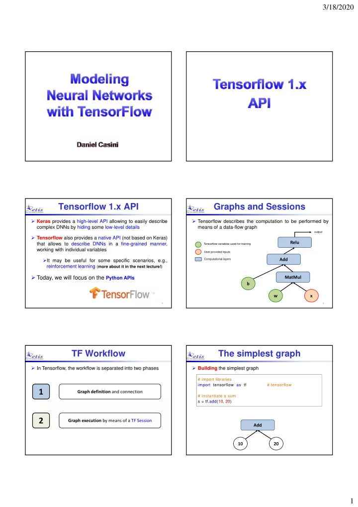
Graphs and Sessions

• Tensorflow describes the computation to be performed by

means of a data-flow graph Relu

Tensorflow variables used for training User provided inputs

• utput

4

Add MatMul w x b

p p Computational layers

TF Workflow

• In Tensorflow, the workflow is separated into two phases

Graph definition and connection

1

Graph execution by means of a TF Session

2 The simplest graph

# import libraries import tensorflow as tf # tensorflow # instantiate a sum tf dd(10 20)

• Building the simplest graph

s = tf.add(10, 20)

Add 10 20

3/18/2020 2

The simplest graph

# import libraries import tensorflow as tf # tensorflow # instantiate a sum s = tf add(10 20)

• Running the simplest graph

s tf.add(10, 20) # create a session object sess = tf.Session() # print the result print sess.run(s) # the output will be 30 # close the session sess.close()

Running a graph

# import libraries import tensorflow as tf # tensorflow # load the dataset s = tf add(10 20)

• The shorter way

s tf.add(10, 20) # create a session object with tf.Session() as sess: # print the result print sess.run(s) # the output will be 30

A more complex graph

# import libraries import tensorflow as tf a=1, b=2, c=3, d=4

• Building and running a more complex graph

Pow

m = tf.multiply(a, b) s = tf.add(c, d) pow = tf.pow(m, s) with tf.Session() as sess: print sess.run(pow)

Add d c Mul b a

Constants

# import libraries import tensorflow as tf # constants definition

• Tensorflow allows to create constants as follows:

Add

c1 = tf.constant(1) c2 = tf.constant(2) s = tf.add(a,b) with tf.Session() as sess: print sess.run(s)

c1 c2

Constants

# import libraries import tensorflow as tf # constants definition

• Tensorflow allows to create constants as follows:

Add

c1 = tf.constant(1) c2 = tf.constant(2) s = tf.add(a,b) with tf.Session() as sess: print sess.run(s)

c1 c2

Constants

# import libraries import tensorflow as tf # constants definition

• Constants and operations can be associated with a name

c1 = tf.constant(1, name =“c1”) c2 = tf.constant(2, name =“c2”) s = tf.add(a, b, name =“sum”) with tf.Session() as sess: print sess.run(s)

Useful for visualize the graph with TensorBoard: more about it later!

3/18/2020 3

Variables

# import libraries import tensorflow as tf

• In Tensorflow, a variable is a special operation that returns

a handle to a persistent mutable tensor that survives across executions of a graph

p # variables definition v1 = tf.Variable(2, name = “scalar”) v2 = tf.Variable([2, 3], name = “array”) v3 = tf.Variable([[2, 3], [1, 0]], name = “matrix”) v4 = tf.Variable(tf.zeros([784, 10]), name = “tensor”)

Variables

# import libraries import tensorflow as tf

• Variables need to be explicitly initialized: there are different ways

Method 1: Initialize all variables at once # variables definition v1 = tf.Variable(2, name = “scalar”) v2 = tf.Variable([2, 3], name = “array”) v3 = tf.Variable([[2, 3], [1, 0]], name = “matrix”) init = tf.global_variables_initializer() with tf.Session() as sess: print sess.run(init)

Variables

# import libraries import tensorflow as tf

• Variables need to be explicitly initialized: there are different ways

Method 2: Initialize only some specific variables # variables definition v1 = tf.Variable(2, name = “scalar”) v2 = tf.Variable([2, 3], name = “array”) v3 = tf.Variable([[2, 3], [1, 0]], name = “matrix”) init2 = tf.variables_initializer([v1, v2]) with tf.Session() as sess: print sess.run(init2)

Variables

# import libraries import tensorflow as tf

• Variables need to be explicitly initialized: there are different ways

Method 3: Initialize a single variable # variables definition v1 = tf.Variable(2, name = “scalar”) v2 = tf.Variable([2, 3], name = “array”) v3 = tf.Variable([[2, 3], [1, 0]], name = “matrix”) with tf.Session() as sess: print sess.run(v3.initializer)

What are Variables for?

• Since variables can be modified at run-time, they are

usually used for the weights and biases of the DNNs

weights = tf.Variable(tf.zeros([400,200]),name="weights") biases = tf Variable(tf zeros([200]) name="biases") biases = tf.Variable(tf.zeros([200]), name= biases ) init = tf.global_variables_initializer() with tf.Session() as sess: sess.run(init)

Variables

weights = tf.Variable(tf.random_normal([400, 200], stddev=0.35), name="weights") bi tf V i bl (tf ([200]) "bi ")

• It may be useful to initialize variables with random values

biases = tf.Variable(tf.zeros([200]), name="biases") init = tf.global_variables_initializer() with tf.Session() as sess: sess.run(init)

3/18/2020 4

Variables

# random initialization with Xavier filler V1 = tf.get_variable("V1", shape=[784, 256], initializer = tf.contrib.layers.xavier_initializer())

• Other common random initializations

with tf.Session() as sess: # print the result sess.run(V1.initializer) x = V1.eval() print(x)

• get_variable return the variable with name "V1“ if

already defined, otherwise creates it

Variables

• Other common random initializations

tf.truncated_normal(shape, mean=0.0, stddev=1.0, dtype=tf.float32, seed=None, name=None) tf.random_uniform(shape, minval=0, maxval=None, dtype=tf.float32, seed=None, name=None) dtype tf.float32, seed None, name None) tf.random_shuffle(value, seed=None, name=None) tf.random_crop(value, size, seed=None, name=None) tf.multinomial(logits, num_samples, seed=None, name=None) tf.random_gamma(shape, alpha, beta=None, dtype=tf.float32, seed=None, name=None)

Variables

weights = tf.Variable(tf.random_normal([784, 200], stddev=0.35), name="weights") i ht 2 tf V i bl ( i ht i iti li d l ()

• Copy a value of a variable into another variable

weights2 = tf.Variable(weights.initialized_value(), name=“weights_copy”)

Assign a Variable

# variables definition v1 = tf.Variable(60, name = “scalar”) v1.assign(120)

• The wrong way

with tf.Session() as sess: sess.run(v1.initializer) print v1.eval()

• What does it print?

It prints 60 because assign is a Tensorflow operation that requires to be executed with sess.run() It prints 60. Why?

Assign a Variable

# variables definition v1 = tf.Variable(60, name = “scalar”) assign_op = v1.assign(120)

• The correct way

with tf.Session() as sess: sess.run(assign_op) print v1.eval()

• What does it print?

It prints 120.

• Note that in this case we don’t need to initialize V1, the

assignment is anyway performed by assign_op

Assign a Variable

v1 = tf.Variable(100, name = “scalar”) assign_op = v1.assign(4 * v1) with tf.Session() as sess: sess.run(v1.initializer)

• More complex assignments

( ) sess.run(assign_op) print v1.eval() sess.run(assign_op) print v1.eval()

• What does it print? 400, and then 1600.
• Note that in this case we need to initialize V1, because

the assignment relies on the initial value of V1.

3/18/2020 5

Save a session

# variables definition v1 = tf.Variable(2, name = “scalar”) v2 = tf.Variable([[2, 3], [1, 0]], name = “matrix”) saver = tf.train.Saver() with tf.Session() as sess: sess.run(init_op) .. # save the variables to disk saver.save(sess, "/tmp/model.ckpt") print("Model saved in file: /tmp/model.ckpt")

Restore a session

# variables definition v1 = tf.Variable(2, name = “scalar”) v2 = tf.Variable([[2, 3], [1, 0]], name = “matrix”) saver = tf.train.Saver() with tf.Session() as sess: # restore the variables to disk saver.restore(sess, "/tmp/model.ckpt") …

More at: https://chromium.googlesource.com/external/github.com/tensorflow/tensorflow/+/r0.7/tensorflow/g3doc/how_tos/variables/index.md

Interactive Session

• An interactive session allows to set the current session as

the default one

• As

a consequence, it is possible to avoid the “with tf.Session() as sess:” command

sess = tf.InteractiveSession() x = tf.constant(600.0) y = tf.constant(2000.0) #This is a short way to define tf.add(a,b) z = a + b print(z.eval()) sess.close()

Placeholders

• In the previous slides, we saw how to model constants,

variables (e.g., for weights and biases)

• What is missing?

We need a way to define Recall y the input variables before knowing the actual values used during execution Placeholders

Placeholders

x = tf.placeholder(tf.float32, shape=[3], name=“x") y = tf.constant(tf.random_normal([3], stddev=0.35)), name=“y") c = tf add(x y) c tf.add(x, y) with tf.Session() as sess: print sess.run(c, {x: [1, 2, 3]}) This is to set values to the placeholder before running the session

Data Types

• Constants, variables and placeholders are associated with a

data type

• Tensorflow data types are similar (and compatible) with

those provided by the numpy library of Python

S l

Data Type Description tf.float32 32 bits floating point tf.float64 64 bits floating points tf.int32 32 bits integer tf.int64 64 bits integer tf.uint16 16 bits unsigned integer tf.string Tensor of byte arrays tf.bool boolean

Some examples:

3/18/2020 6

Data Types

• Compatibility with numpy:

tf.int32 == np.int32

• Tensorflow and numpy types can be used interchangeably

TRUE

x = tf.placeholder(numpy.int32, shape=[400, 200]) y = tf.placeholder(tf.int32, shape=[400, 200])

32

TensorBoard

• TensorBoard is the Tensorflow visualization toolkit,

which allows to:

• show the operations and layers composing a graph
• view histograms of weights and biases as they change over

time time

• profile Tensorflow applications
• keep track of metrics (e.g., loss and accuracy)

TensorBoard TensorBoard

• There is no need to install TensorBoard, it is included in the

default Tensorflow installation

• To visualize data with TensorBoard, we need to specifically

instrument the code to do this (we’ll see how next)

• O

th d t h b l d b T fl

• Once

the data has been logged by

• ur

Tensorflow application, let’s say in a directory named “graph“ we can launch TensorBoard by typing in a terminal:

C:\User> tensorboard ‐‐logdir graph

• TensorBoard will be available in your browser at the address

localhost:6006

Using TensorBoard

• Let’s focus on the graph visualization functionality of

TensorBoard

tf t t(5 0) a = tf.constant(5.0) b = tf.constant(6.0) c = a * b s = tf.add(a, c) with tf.Session() as sess: print(sess.run(s)) writer = tf.summary.FileWriter('./graph', sess.graph)

3/18/2020 7

Using TensorBoard

tf t t(5 0) Default TensorFlow names

• Let’s focus on the graph visualization functionality of

TensorBoard

screenshot from TensorBoard

a = tf.constant(5.0) b = tf.constant(6.0) c = a * b s = tf.add(a, c) with tf.Session() as sess: print(sess.run(s)) writer = tf.summary.FileWriter('./graph', sess.graph)

Using TensorBoard

tf t t(5 0 " ")) Better names

screenshot from TensorBoard

a = tf.constant(5.0, name="a")) b = tf.constant(6.0, name="b")) c = a * b s = tf.add(a, c) with tf.Session() as sess: print(sess.run(s)) writer = tf.summary.FileWriter('./graph', sess.graph)

39

Example

• Next, we’ll see how to build and train a simple network using

Tensorflow

• To keep the example simple without relying on the usual

and super-popular examples on image recognition, suppose to build a network to forecast the number of infections due to Covid-19 in the next days

• Of course, the problem is very complex and depends on a

lot of variables, but we’ll consider just a very simple dependency

64

L1

1

X

64

L2 FC FC

Y

1

Input Output

Example: Covid-NN

Size Description Input 1 integer Number of days from Feb 22 Layer L1 64 neurons Fully connected Layer L2 64 neurons Fully connected Output 1 integer Number of infected people in Italy at day X

Covid-NN in Tensorflow

# import libraries import tensorflow as tf import numpy

• Step 1: import libraries and define parameters

import os # parameters learning_rate = 0.22

3/18/2020 8

Covid-NN in Tensorflow

# training inputs: days from Feb 22 to Mar 12 train_X = numpy.asarray([1, 2, 3, 4, 5, 6, 7, 8, 9, 10, 11, 12, 13, 14, 15, 16, 17, 18, 19]) # reshape the array size t i X t i X h (19 1)

• Step 2: define the (small) training set

train_X = train_X.reshape(19,1) # training outputs: infected people train_Y = numpy.asarray([76, 148, 222, 311, 385, 588, 821, 1049, 1577, 1835, 2263, 2706, 3296, 3916, 5061, 7375, 8878, 10149, 12462]) # reshape the array size train_Y = train_Y.reshape(19,1)

Covid-NN in Tensorflow

# Network Parameters # number of neurons 1st hidden layer n_hidden_1 = 64 # b f 2 d hidd l

• Step 3: define the network parameters

# number of neurons 2nd hidden layer n_hidden_2 = 64 # days size_input = 1 # number of cases size_output = 1

Covid-NN in Tensorflow

# placeholders X = tf.placeholder(tf.float32, [None, size_input]) Y = tf.placeholder(tf.float32, [None, size output])

• Step 4: define the inputs (placeholders)

p ( , [ , _ p ])

Covid-NN in Tensorflow

# weights and biases weights = { 'h1': tf.Variable(tf.random_normal([size_input, n_hidden_1])), 'h2': tf.Variable(tf.random normal([n hidden 1, n hidden 2])),

• Step 5: define weights and biases

Python Dictionary ( _ ([ _ _ , _ _ ])), 'out': tf.Variable(tf.random_normal([n_hidden_2, size_output])) } biases = { 'b1': tf.Variable(tf.random_normal([n_hidden_1])), 'b2': tf.Variable(tf.random_normal([n_hidden_2])), 'out': tf.Variable(tf.random_normal([size_output])) } Python Dictionary

Covid-NN in Tensorflow

# hidden fully connected layer layer_1 = tf.add(tf.matmul(X, weights['h1']), biases['b1']) # hidden fully connected layer layer 2 = tf.add(tf.matmul(layer 1, weights['h2']), biases['b2'])

• Step 6: build the network

y _ ( ( y _ , g [ ]), [ ]) # output layer

• ut_layer = tf.add(tf.matmul(layer_2, weights['out']), biases['out'])

Covid-NN in Tensorflow

# loss and optimizer fun = tf.nn.softmax_cross_entropy_with_logits(logits=out_layer, labels=Y) loss_op = tf.reduce_mean(fun)

• Step 7: initializations
• ptimizer = tf.train.AdamOptimizer(learning_rate=learning_rate)

train_op = optimizer.minimize(loss_op) # variable initializer init = tf.global_variables_initializer()

3/18/2020 9

Covid-NN in Tensorflow

with tf.Session() as sess: # run the initializer sess.run(init)

• Step 8: train and infere the network

( ) #train the network sess.run(train_op, feed_dict={X: train_X, Y: train_Y}) #infere the network print(sess.run(out_layer, feed_dict={X: prediction_X}))

Covid-NN in Tensorflow

• Output*:

[[18061.268] [18958.889] [19856.508] [20754.13 ] [21651 748]

• The output is ‘realistic’ but note that

many changes may be done to improve this network

[21651.748] [22549.37 ] [23446.99 ] [24344.613] [25242.234] [26139.855] [27037.475]]

• This is just a didactic example

*The network output may change run-by-run as an effect of the random initialization of the weights and the small training set

Covid-NN in Tensorflow

• Some suggestions for improvements:
• Train the network with the Wuhan data set
• ‘Play’ with the number of neurons, number of layers, activation

functions, etc.

• Change the input of the network, e.g., use sequences of inputs

instead of a single input (it may help the network to learn better how sequences behaves)

• Some references for the data sets:

[1] https://github.com/CSSEGISandData/COVID19/tree/master/csse_covid_19_data [2] https://www.worldometers.info/coronavirus/

Covid-NN in Tensorflow Covid-NN in Tensorflow

placeholders

Covid-NN in Tensorflow

weights

3/18/2020 10

Covid-NN in Tensorflow

random initialization

Covid-NN in Tensorflow

biases

Covid-NN in Tensorflow

layers

Covid-NN in Tensorflow

Training parameters and operations

59

Mid-level TF APIs High-level TF APIs

Layers Datasets Losses Estimators Keras TF learn Metrics TF-sim

The TensorFlow Stack

     

Hardware Operating Systems TensorFlow Distributed Execution Engine Python Frontend C++ TF runtime Language

60

CPU GPU TPU

Windows Linux Android iOS

     

DSP

3/18/2020 11

Example

• When multiple devices are available (e.g., a CPU and

multiple GPUs), TensorFlow offers a Python API to spread the computation of a TensorFlow graph over multiple devices.

• This may help improving the performance.
• Next we’ll focus on an example assuming to have 2 GPUs
• Next, we’ll focus on an example, assuming to have 2 GPUs

and 1 CPU. Some remarks:

• Note that Tensorflow refers to the term ‘CPU’ by considering a group
• f cores
• It does not identify processor cores individually (at least with the

high-level of Python API)

• Internally to

each core, it implements a complex scheduling mechanisms based on pools of threads

Example

• Consider this network

import tensorflow as tf # constants a = tf.constant(5.0, name = "a") b = tf.constant(6.0, name = "b") c = tf.constant(10.0, name = "c") d = tf.constant(20.0, name = "d")

Example

sum = tf.add(a, b, name="fork") mul = tf.multiply(sum, b, name = "child_1") mul2 = tf.multiply(sum, c, name = "child_2")

• Consider this network

mul3 = tf.multiply(sum, d, name = "child_3") sum2 = tf.add(mul, mul2, name = "join") sum3 = tf.add(sum2, mul3, name = "join_2") with tf.Session() as sess: writer = tf.summary.FileWriter('./graph', sess.graph) print(sess.run(sum3))

Example Example Example

These nodes are parallel, we may think of making them running on different devices to enhance parallelism

3/18/2020 12

Partitioning

CPU GPU_1 GPU_2

Partitioning

import tensorflow as tf #global operation names visible from all devices sum = [] mul2 = [] mul3 = [] # constants a = tf.constant(5.0, name = "a") b = tf.constant(6.0, name = "b") c = tf.constant(10.0, name = "c") d = tf.constant(20.0, name = "d")

Partitioning

with tf.device('/cpu:0'): sum = tf.add(a, b, name="fork") mul = tf.multiply(sum, b, name="child_1") sum2 = tf.add(mul, mul2, name="join") sum3 = tf.add(sum2, mul3, name="join_2")

More examples at: https://gist.github.com/j-min/baae1aa56e861cab9831b3722755ae6d

with tf.device('/gpu:0'): mul2 = tf.multiply(sum, c, name="child_2") with tf.device('/gpu:1'): mul3 = tf.multiply(sum, d, name = "child_3") sess = tf.Session() print(sess.run(mul3))

Multi-Device Tensorflow

• If no partitioning is specified, Tensorflow automatically uses

the available resources by means of a default partitioning algorithm

• This is enough in most of the cases
• However for very computationally expensive graphs it may
• However, for very computationally-expensive graphs it may

be worth to investigate different allocations

More at: https://www.tensorflow.org/guide/distributed_training

71

Eager API

• A different Tensorflow API, introduced in 2017, allowing to

run operations immediately as they are called by Python, without specifying session.run()

• More intuitive
• Easier to debug
• Easier to debug
• Better for specifying dynamic models
• Most of the API remains the same with or without Eager

execution enabled

3/18/2020 13

Enabling Eager API

import numpy as np import tensorflow as tf import tensorflow.contrib.eager as tfe

• Eager execution can be specified as follows

# set Eager API print("Setting Eager mode...") tfe.enable_eager_execution()

Eager API Example

# constants a = tf.constant(2) b = tf.constant(3) # we can print them immediately, without session.run() print("a = %i" % a) print("b = %i" % b)

Eager API Example

# define and run operations without tf.session() c = a + b print("a + b = %i" % c) d = a * b print("a * b = %i" % d) p ( )

76 From: https://github.com/aymericdamien/TensorFlow-Examples/blob/master/examples/3_NeuralNetworks/neural_network_eager_api.py

Eager API Example

L1 L2 FC FC

Input: MNIST Images Output: MNIST Classes

256 28x28

X

256

FC FC

Y

10

Eager API Example

# Import Tensorflow import tensorflow as tf # Import MNIST data

• Step 1: import libraries, enable eager execution and load

the data set

from tensorflow.examples.tutorials.mnist import input_data # Set Eager API tf.enable_eager_execution() tfe = tf.contrib.eager mnist = input_data.read_data_sets("/tmp/data/")

3/18/2020 14

Eager API Example

# Parameters learning_rate = 0.001 num_steps = 1000

• Step 2: define the network parameters

batch_size = 128 display_step = 100 # Network Parameters n_hidden_1 = 256 # 1st layer number of neurons n_hidden_2 = 256 # 2nd layer number of neurons num_input = 784 # MNIST data input (img shape: 28*28) num_classes = 10 # MNIST total classes (0-9 digits)

Eager API Example

# Using TF Dataset to split data into batches dataset = tf.data.Dataset.from_tensor_slices( (mnist.train.images, mnist.train.labels))

• Step 2: split the data set into batches

dataset = dataset.repeat().batch(batch_size).prefetch(batch_size) dataset_iter = tfe.Iterator(dataset)

prefetch allows the CPU loading the data when the GPU is executing other

• perations

batch extracts batches from training in groups of size batch_size repeat repeats the element of the dataset to allow the extraction of batches

Eager API Example

class NeuralNet(tfe.Network): def __init__(self): (N lN t lf) i it ()

• Step 3: define the Neural Network using a Python class,

required to use the Eager API and tf.layers together

super(NeuralNet, self).__init__() # Hidden fully connected layer with 256 neurons self.layer1 = self.track_layer( tf.layers.Dense(n_hidden_1, activation=tf.nn.relu)) # Hidden fully connected layer with 256 neurons self.layer2 = self.track_layer( tf.layers.Dense(n_hidden_2, activation=tf.nn.relu)) # Output fully connected layer with a neuron for each class self.out_layer = self.track_layer(tf.layers.Dense(num_classes))

Eager API Example

class NeuralNet(tfe.Network): … # previous slide

• Step 4: the class must implement the __init__ and call

methods

def call(self, x): x = self.layer1(x) x = self.layer2(x) return self.out_layer(x)

Eager API Example

# Cross-Entropy loss function def loss_fn(inference_fn, inputs, labels): # U i ft t

• Step 5: define the loss function as a Python function

# Using sparse_softmax cross entropy return tf.reduce_mean( tf.nn.sparse_softmax_cross_entropy_with_logits( logits=inference_fn(inputs), labels=labels))

Eager API Example

# Calculate accuracy def accuracy_fn(inference_fn, inputs, labels): di ti tf ft (i f f (i t ))

• Step 6: define the accuracy function as a Python function

prediction = tf.nn.softmax(inference_fn(inputs)) correct_pred = tf.equal(tf.argmax(prediction, 1), labels) return tf.reduce_mean(tf.cast(correct_pred, tf.float32))

3/18/2020 15

Eager API Example

neural_net = NeuralNet()

# SGD Optimizer

• Step 7: create an instance of the network and specify the
• ptimizer parameters

# SGD Optimizer

• ptimizer = tf.train.AdamOptimizer(learning_rate=learning_rate)

# Compute gradients grad = tfe.implicit_gradients(loss_fn)

Eager API Example

average_loss = 0. average_acc = 0.

• Step 8: train the network (1)

for step in range(num_steps): # Iterate through the dataset d = dataset_iter.next()

Eager API Example

for step in range(num_steps): # previous slide

• Step 8: train the network (2)

… # previous slide # Images x_batch = d[0] # Labels y_batch = tf.cast(d[1], dtype=tf.int64)

Eager API Example

for step in range(num_steps): … # previous slide # Compute the batch loss b t h l l f ( l t b t h b t h)

• Step 8: train the network (3)

batch_loss = loss_fn(neural_net, x_batch, y_batch) average_loss += batch_loss # Compute the batch accuracy batch_accuracy = accuracy_fn(neural_net, x_batch, y_batch) average_acc += batch_accuracy # Update the variables following gradients info

• ptimizer.apply_gradients(grad(neural_net, x_batch, y_batch))

Eager API Example

for step in range(num_steps): … # previous slide # Display info

• Step 8: train the network (4)

if (step + 1) % if step > 0: average_loss /= display_step average_acc /= display_step print("Step:", '%04d' % (step + 1), " loss=", "{:.9f}".format(average_loss), " accuracy=", "{:.4f}".format(average_acc)) average_loss = 0. average_acc = 0.

Eager API Example

# Evaluate model on the test image set testX = mnist.test.images testY = mnist test labels

• Step 8: evaluate the accuracy of the network

testY = mnist.test.labels test_acc = accuracy_fn(neural_net, testX, testY) print("Testset Accuracy: {:.4f}".format(test_acc))

3/18/2020 16

91

TensorFlow 2

• Easier to use, many contrib layers have been merged into

Tensorflow, others have been removed

• Eager execution by default
• Placeholders are not needed anymore
• Tutorials

are available about how to migrate a Tensorflow 1.X network to Tensorflow 2

• Examples are available here:

https://www.tensorflow.org/guide/migrate https://github.com/aymericdamien/TensorFlow-Examples/tree/master/tensorflow_v2

References

• https://github.com/sujaybabruwad/LeNet-in-Tensorflow/blob/master/LeNet-Lab.ipynb
• https://github.com/aymericdamien/TensorFlow-

Examples/blob/master/examples/3_NeuralNetworks/neural_network_eager_api.py

T hank hank yo u! yo u!

Danie l Casini Danie l Casini danie l.c asini@sssup.it danie l.c asini@sssup.it