TCP Congestion Control: Algorithms and Analysis Simon S. Lam - - PDF document

1

TCP Congestion Control: Algorithms and Analysis

Simon S. Lam Department of Computer Sciences Department of Computer Sciences The University of Texas at Austin

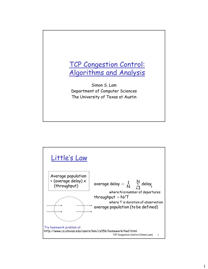
Little’s Law

Average population g p p = (average delay) x (throughput)    

where N is number of departures where T is duration of observation

N

1 average delay delayi N i 1 throughput N/T average population (to be defined)

2

average population (to be defined)

Try homework problem at http://www.cs.utexas.edu/users/lam/cs356/homework/hw2.html

TCP Congestion Control (Simon Lam)

2

in system n(t) Time t Number

3

 

T

dt t n T ) ( 1 population average

TCP Congestion Control (Simon Lam)

Sliding Window Protocol

 Consider an infinite array, Source, at the

sender, and an infinite array, Sink, at the receiver.

1 2 a–1 a s–1 s send window acknowledged unacknowledged Source: P1 Sender 1 2 r received delivered receive window r + RW – 1 Sink: P2 Receiver next expected RW receive window size SW send window size (s - a  SW) 4 TCP Congestion Control (Simon Lam)

3

Sliding Windows in Action

 Data unit r has just been received by P2

 Receive window slides forward

P d l k h

 P2 sends cumulative ack with sequence

number it expects to receive next (r+3)

unacknowledged 1 2 a–1 a s–1 s send window acknowledged Source: P1 Sender 1 2 r delivered receive window r + RW – 1 Sink: P2 Receiver next expected r+3 5 TCP Congestion Control (Simon Lam)

Sliding Windows in Action

 P1 has just received cumulative ack with

r+3 as next expected sequence number

 Send window slides forward

1 2 a–1 a s–1 s send window acknowledged Source: P1 Sender 1 2 r delivered receive window r + RW – 1 Sink: P2 Receiver next expected 6 TCP Congestion Control (Simon Lam)

4

Window Flow Control

RTT

time time Source Destination 1 2 W 1 2 W 1 2 W data ACKs 1 2 W

7

 ~ W packets per RTT when no loss  Lost packet detected by missing ACK

(note: timeout value TO > RTT)

time

TCP Congestion Control (Simon Lam)

Throughput (send rate)

 Limit the number of unacked transmitted

packets in the network to window size W

 Throughput packets/sec

= bytes/sec

W RTT 

W MSS RTT 

8

 Where did we apply Little’s Law? Answer: Consider send buffer

TCP Congestion Control (Simon Lam)

5

Clarifications

 Average number in the send buffer is typically

less than W unless packet arrival rate to send buffer is infinite -> previous formula provides a throughput upper bound throughput upper bound

 If each packet may be lost with rate p, then the

average delay is Since TO > RTT, actual throughput is smaller.

 With loss, goodput is

(1 )

O

p RTT p T    

(1 ) th h t 

9

g p

 Note: in some papers and other context (e.g., random

access protocols), goodput is called throughput. To avoid confusion, throughput is called send rate

(1 ) p throughput  

TCP Congestion Control (Simon Lam)

Effect of Congestion

 W too big for each of many flows -> congestion  Packet loss -> transmissions on links prior to packet

loss are wasted loss are wasted

 Congestion collapse due too many retransmissions

and too much waste

 October 1986, Internet had its first congestion

collapse

goodput

10

load

TCP Congestion Control (Simon Lam)

6

TCP Window Control

 Receiver flow control

 Avoid overloading receiver  Avoid overloading receiver  rwnd:

receiver (advertised) window

 Receiver sends rwnd to sender

 Network congestion control

 Sender tries to avoid overloading network  It infers available network capacity from “loss

i di ti ”

11

indications”

 cwnd:

congestion window  Sender sets W = min (cwnd, rwnd)

TCP Congestion Control (Simon Lam)

Receiver Flow Control

 Receiver advertises rwnd with each packet it

sends sends

 Size of rwnd indicates available space in

receive buffer

 decreased when data is received from IP layer and

ack’d

 increased when data is consumed by application

12

 increased when data is consumed by application

process

TCP Congestion Control (Simon Lam)

7

Network Congestion Control

 Sender calculates cwnd from indications of

network congestion

 Congestion indications  Congestion indications

 timeout (loss)  dupACK (loss likely)  queueing delay  mark (needs ECN)

 TCP algorithms to calculate cwnd

13

 Tahoe, Reno, Vegas, …

 Link algorithms:

 RED, REM …

TCP Congestion Control (Simon Lam)

TCP & AQM

pl(t) xi(t) pl( )

Congestion measures pl(t) for distributed feedback control of xi(t)

14

Congestion measures pl(t) for distributed feedback control of xi(t)

 loss and dupACK (DropTail)  queueing delay (Vegas)

with the help of active queue management (AQM)

 queue length (RED)  price (REM) TCP Congestion Control (Simon Lam)

8

TCP Congestion Control

 Tahoe (Jacobson 1988)

 Slow Start  Congestion Avoidance

F t R t it

 Fast Retransmit

 Reno (Jacobson 1990)

 Fast Recovery  Its variants: NewReno, SACK

 Vegas (Brakmo & Peterson 1994)

 New Congestion Avoidance

 AQM E (Fl d & b 1 )

15  RED (Floyd & Jacobson 1993)

• Probabilistic marking or dropping

 REM (Athuraliya & Low 2000)

• Clear buffer, match rate

 Others…

TCP Congestion Control (Simon Lam)

Slow Start

 Start with cwnd = 1  On each successful ACK, increment cwnd

cwnd  cwnd + 1 cwnd  cwnd + 1

 Exponential growth of cwnd

each RTT: cwnd  2 x cwnd

 Enter CA when cwnd >= ssthresh  For initial slow start, ssthresh is set to a very large

16

, y g value (e.g., 65 Kbytes) Note: for clarity, cwnd, rwnd, and ssthresh are counted in packets (segments) rather than in bytes

TCP Congestion Control (Simon Lam)

9

Slow Start

receiver sender

cwnd

1

data packet ACK

1 RTT

1 2 3 4

17

5 6 7 8

cwnd  cwnd + 1 (for each ACK)

TCP Congestion Control (Simon Lam)

Congestion Avoidance

 CA starts when

cwnd  ssthresh

cwnd

1

receiver sender

cwnd  ssthresh

 On each successful

ACK: cwnd  cwnd + 1/cwnd

1 2 3

1 RTT

data packet ACK

18

 Linear growth of cwnd

each RTT: cwnd  cwnd + 1

4

TCP Congestion Control (Simon Lam)

10

Packet Loss

 Assumption: loss indicates congestion  P

k t l d t t d b

 Packet loss detected by

 Retransmission timeout (RTO timer)  Duplicate ACKs (at least 3)

1 2 3 4 5 6

Packets

7

19

1 2 3 4 5 6 1 2 3

Acknowledgements

3 3 7 3

TCP Congestion Control (Simon Lam)

Fast Retransmit

 A timeout is quite long (> RTT)  Upon receiving 3 dupACKs, immediately

p g p , y retransmit without waiting for timeout

 Adjusts ssthresh

ssthresh  max(flightsize/2, 2)

h fli htsiz is numb f utst ndin p ck ts

20

where flightsize is number of outstanding packets, which may be less than W = min(rwnd, cwnd)  Enter Slow Start (cwnd = 1)

TCP Congestion Control (Simon Lam)

11

TCP Tahoe (Jacobson 1988)

cwnd time

21

SS time (in RTTs) CA SS: Slow Start CA: Congestion Avoidance

TCP Congestion Control (Simon Lam)

Successive Timeouts

 When there is another timeout, double the

timeout value

 Keep doing so for each additional loss-  Keep doing so for each additional loss-

retransmission

 Exponential backoff up to

max timeout value equal to 64 times initial timeout value

22

Note: red line in figure denotes a loss indication

TCP Congestion Control (Simon Lam)

12

Summary: Tahoe

 Basic ideas

 Probe network for spare capacity during SS and

CA and increase send rate CA and increase send rate

 Drastically reduce rate on congestion indication  Self-clocking  Error recovery by retransmission  Round trip time estimation (to get TO value)

f or ever y ACK { i f ( W < sst hr esh) t hen W ++ ( SS)

23

i f ( W < sst hr esh) t hen W ++ ( SS) el se W += 1/ W ( CA) } f or ever y l oss i ndi cat i on { sst hr esh = W / 2 W = 1 }

TCP Congestion Control (Simon Lam)

TCP Tahoe (Jacobson 1988)

cwnd time

24

SS CA SS: Slow Start CA: Congestion Avoidance

TCP Congestion Control (Simon Lam)

13

TCP Reno (Jacobson 1990)

cwnd time

25

SS CA SS: Slow Start CA: Congestion Avoidance Fast retransmission/fast recovery

TCP Congestion Control (Simon Lam)

TCP Reno (another scenario)

TO halved 3 dupACKs cwnd

26

Initial slow start

t

Slow start until cwnd reaches ssthresh

TCP Congestion Control (Simon Lam)

14

Fast recovery (in detail)

 Idea: each dupACK represents a packet

successfully received Therefore no need for successfully received. Therefore, no need for very drastic action

 Enter FR/FR after 3 dupACKs

 Set ssthresh  max(flightsize/2, 2)  Retransmit lost packet  Set cwnd  ssthresh + #dupACKs (window inflation)  Wait till W=min(rwnd cwnd) is large enough; transmit 27  Wait till W=min(rwnd, cwnd) is large enough; transmit

new packet(s)

 On non-dup ACK (1 RTT later), set cwnd  ssthresh

(window deflation)  Enter CA

TCP Congestion Control (Simon Lam)

9

Example: FR/FR

time S 1 2 3 4 5 6 8 7 1 10 11

9 4

 Above scenario: Packet 1 is lost, packets 2, 3, and

4 i d d ACK i h d

time R 8

cwnd 8 ssthresh 7 4

Exit FR/FR

4 4 4 11

28

p 4 are received; dupACKs with seq. no. 0 returned

 Fast retransmit

 Retransmit on 3 dupACKs

 Fast recovery

 Inflate window such that new packets 9, 10, and 11 can be

sent while repairing loss

TCP Congestion Control (Simon Lam)

15

Summary: Reno

 Basic ideas

 Fast recovery avoids slow start  Fast recovery avoids slow start  dupACKs: fast retransmit + fast recovery  Timeout: fast retransmit + slow start congest i on FR/ FR dupACKs

29

sl ow st ar t r et r ansm i t avoi dance FR/ FR t i m eout

TCP Congestion Control (Simon Lam)

AIMD in steady state

multiplicative decrease: cut cwnd in half after 3 dupACKs additive increase: increase cwnd by 1 MSS every RTT in the bs f l ss

16 Kbytes 24 Kbytes congestion window

absence of any loss event

30

8 Kbytes time

Long-lived TCP connection

TCP Congestion Control (Simon Lam)

16

TCP throughput (send rate)

 We derived the approximate formula

throughput = packets/sec

 W changes with the arrival of each

congestion indication l l ( ) d d W RTT

31

 To calculate (average) send rate, we need

the average value of W Q: W is a function of what parameter?

TCP Congestion Control (Simon Lam)

First approximation

• M. Mathis, et al., “The Macroscopic Behavior of the TCP Congestion

Avoidance Algorithm,”ACM Computer Communicatons Review, 27(3), 1997.

 No slow-start, no timeout, long-lived TCP

connection connection

 Independent identically distributed “periods”  Each packet may be lost with probability p

32 TCP Congestion Control (Simon Lam)

17

Geometric Distribution

• Ave. no. of transmissions to get first loss

1 1 1

(1 )i

i i i

n ib i p p

    

  

 

1 1 1 2

(1 ) (1 ) (1 ) 1 1 1 1

i i i i i i

p i p d d p p p p dp dp d p p dp p p

      

            

  

33

1 1 1/ dp p p p   Similarly, ave. no. of transmissions to get first success is 1/(1-p)

TCP Congestion Control (Simon Lam)

First approximation (cont.)

8 3 W p   Average number of packets delivered in

• ne period (area under

2 2 2

1 3 2 2 2 8 W W W              

2

send rate (in packets/sec) 3

• no. of packets/period

8 time per period 2 W W RTT        

• ne period (area under
• ne saw-tooth)

 Average number of k i d

34

2 1/ 1 3 2 2 3 p RTT p RTT p           packets sent per period (incl. loss at the end) is 1/p  Equating the two and solving for W, we get

TCP Congestion Control (Simon Lam)

18

TCP ACK generation [RFC 1122, RFC 2581]

Event at Receiver TCP Receiver action

Arrival of in-order segment with expected seq #. All data up to expected seq # already ACKed Arrival of in-order segment with expected seq #. One other segment has ACK pending Arrival of out of order segment Delayed ACK. Wait up to 500ms for next segment. If no next segment, send ACK Immediately send single cumulative ACK, ACKing both in-order segments Immediately send duplicate ACK

35

Arrival of out-of-order segment higher-than-expect seq. # . Gap detected Arrival of segment that partially or completely fills gap Immediately send duplicate ACK, indicating seq. # of next expected byte Immediate send ACK, provided that segment starts at lower end of gap

TCP Congestion Control (Simon Lam)

Receiver implements Delayed ACKs

 Receiver sends one ACK for every two packets

received -> each saw-tooth is WxRTT wide h

• > area under a saw-tooth is

 Send rate is  One ACK for every b packets received -> send rate

i

2

3 4 W

1 3 4 RTT p

36

is

1 3 2 RTT bp

TCP Congestion Control (Simon Lam)

19

M d li TCP Th h t A Si l Modeling TCP Throughput: A Simple Model and its Empirical Validation,

• Proc. ACM SIGCOMM, 1998

Jitendra Padhye, Victor Firoiu, D T l d Ji K Don Towsley, and Jim Kurose

Motivation

 Previous formulas not so accurate when

loss rates are high loss rates are high

 TCP traces show that there are more loss

indications due to timeouts (TO) than due to triple dupACKs (TD)

38 TCP Congestion Control (Simon Lam)

20

Objectives

 More accurate steady-state throughput

formula as a function of loss rate and RTT formula as a function of loss rate and RTT by also accounting for TO behavior of a TCP connection

 Formula applicable over a wider range of

loss rates

 Explicit statements of assumptions and

i ti d i d i ti f

39

approximations used in derivation of throughput formula

 Formula to include the impact of a small

rwnd

TCP Congestion Control (Simon Lam)

Many assumptions and approximations

 A1. TCP sender is saturated, i.e., source

application process always has a packet to application process always has a packet to send when send window has space available

 i.e., bulk transfer application

 A2. Slow Start not modeled  A3. Time to send all packets in a window is

smaller than RTT

40

smaller than RTT

 i.e.,transmission rate is not too low

TCP Congestion Control (Simon Lam)

21

• A3. Time to send W packets is

less than RTT

Start of round

• ACK reception

marks the end of current round and time

Start of round

beginning of next round.

• Approximation: For

b > 1, ACK is not received immediately after

41

End of round space

immediately after

• ne RTT, but it is so

assumed in the analysis

TCP Congestion Control (Simon Lam)

AIMD evolution of Window Size over time

 Each TD period is ended by a TD loss indication.  TDPi period has duration Ai rounds

42

i p i

 A4. Duration of a round (RTT) is independent of

window size

 approximation (poor for a slow line)

 A5. No window inflation in Fast Recovery

 approximation TCP Congestion Control (Simon Lam)

22

Markov regenerative assumption

 For the i-th TD period, Wi is window size at

the end of the period, Yi is the number of packets sent in the period

 A6. Assume {Wi} to be a Markov

regenerative process with rewards {Yi}

 Given A6, the steady-state TCP throughput

is

[ ] [ ] N E Y E Y

43

[ ] [ ] lim lim [ ] [ ]

t i t t t i

N E Y E Y B B t E A E A

 

   

TCP Congestion Control (Simon Lam)

Consider i-th TD period

when ACK of last packet is received

44

 One ACK after receiving b packets (b = 2 in above

figure) -> linear increase has a slope of 1/b packet per RTT

 Number of rounds is Xi +1

 i is the first packet lost in i-th TD period

TCP Congestion Control (Simon Lam)

23

Loss assumptions

 A7. Losses in different rounds are

independent independent

 approximation

 A8. Losses within the same round are

correlated as follows: If a packet is lost, all remaining packets transmitted until the end of that round are also lost

i ti b t l b h i b t l

45

 approximation – bursty loss behavior but only

within the same round

 all lost packets in the same round are counted

as a single loss indication when estimating p

TCP Congestion Control (Simon Lam)

AIMD throughput derivation (1)

• seq. no. of first loss

r round trip time Y no. of packets sent

[ ] 1/ [ ] 1 E p E r RTT   



p W window size X no. of rounds A time duration of a period

1

1 [ ] [ ] [ ] 1 1 [ ] From , we have 2 [ ] [ ] 2

i i i

E Y E E W E W p W X W b b E X E W b 



        

46

<- from A4 that round trip times are independent of Wi

[ ] ( [ ] 1) [ ] ( [ ] 1) 2 1 1 [ ] [ ] send rate [ ] ( [ ] 1) 2 b E A E X E r E W RTT E W E Y p B b E A E W RTT         

TCP Congestion Control (Simon Lam)

24

AIMD throughput derivation (2)

Another way to compute E[Y]

/ 1 1

( ) 2

i

X b i i i k

W Y k b 

  

  



<- A9. Assume that

1 1

( 1) 2 2 ( 1) 2 2 Let [ ] be [ ] and we have 2

i i i i i i i i i

X W X X b X W W W E E   

 

       

47

{Xi} and {Wi} are mutually independent i.i.d. sequences of random variables

[ ] [ ] [ ] ( [ ] 1) [ ] 2 2 [ ] [ ] ( [ ] 1) [ ] 4 2 2 E X E W E Y E W E bE W E W W E W E         

TCP Congestion Control (Simon Lam)

AIMD throughput (3)

 Equate the two previous formulas for E[Y]. Solve the quadratic

equation with E[W] as the only unknown

1 [ ] 1 [ ] E Y E W   

2

[ ] 1 [ ] [ ] [ ] ( [ ] 1) [ ] 4 2 2 2 8(1 ) 2 [ ] ( ) 3 3 3 E Y E W p bE W E W W E W E b p b E W b bp b           

48

3 3 3 1 [ ] send rate ( ) [ ] b bp b p E W p B p E A   

TCP Congestion Control (Simon Lam)

25

AIMD throughput (4)

To get a simple formula, collect terms that are o(1/sqrt(p))

8 [ ] (1/ ) 3 2 [ ] [ ] (1/ ) 2 3 1/ (1/ ) 1 3 send rate ( ) (1/ ) E W

• p

bp b b E X E W

• p

p p o p B p

• p

        

49

send rate ( ) (1/ ) 2 2 (1/ ) 3 B p

• p

RTT bp b RTT

• p

p          

TCP Congestion Control (Simon Lam)

AIMD with TO

 Let ni denote the number of TD periods within a

cycle ending in i-th TO period, Ri denote no. of

50

cycle ending in i th TO period, Ri denote no. of retransmissions in i-th TO period

 A10. {ni } form an i.i.d. sequence, independent of

{Yij} and {Aij}

TCP Congestion Control (Simon Lam)

26

Throughput of AIMD with TO (1)

[ ] [ ] [ ] [ ] [ ] [ ] [ ] [ ] [ ] [ ] [ ] [ ]

TO

E M E n E Y E R E S E n E A E Z E M E E Y E R     Assumption of Markov regenerative [ ] [ ] [ ] [ ] send rate [ ] [ ] [ ] [ ] [ ] [ ] [ ] [ ] 1 where [ ]

TO TO

E M E n E Y E R B E S E n E A E Z E Y Q E R B E A Q E Z Q E           process again. P b bilit th t

51

[ ] 1 [ ] 1 with and [ ] to be determined

TO

E n E R p Q E Z   <- Probability that a given loss indication is a TO

TCP Congestion Control (Simon Lam)

Approximate solution for Q

52

A given loss indication is a TO is the union of two events Two or less acked packets in penultimate round or two or less acked packets in final round

TCP Congestion Control (Simon Lam)

27

Approximate solution for Q (cont.)

<- penultimate round of w packets, first k packets ack’d given there is a loss (1 ) ( , ) 1 (1 )

k w

p p A w k p     <- for last round, k packets sent, m packets ack’d in sequence <- at most 2 dupACKs



( , ) (1 ) , 1 ( , ) (1 ) , ( ) 1 if 3

m m

C k m p p m k C k m p m k Q w w         

53

p <- probability of fewer than 3 packets sent successfully in penultimate round or less than 3 acks in last round

2 2 3

( ) ( , ) ( , ) ( , ) if 4

w k k m

Q A w k A w k C k m w

  

  

  

TCP Congestion Control (Simon Lam)

Approximate solution for Q (cont.)

54

 Q is

But we don’t know the probability distribution of Wi

 Approximation 

3 3 ( [ ]) min(1, ) min(1,3 ) [ ] 8 bp Q Q E W E W    

[ ( )] E Q w

TCP Congestion Control (Simon Lam)

28

Throughput of AIMD with TO (2)

1

[ ] (1 ) for 1,2,... (2 1) for 6

k k k O

P R k p p k L T k



      

<- duration of k TOs in a row

2 3 4 5 6 2

(63 64( 6)) for 7 1 2 4 8 16 32 [ ] 1 ( ) (1 32 ) 1 [ ] [ ] d ( )

O TO O O

k T k p p p p p p E Z T p f p T T p p E Y Q E R B                  

<- approximation

55

[ ] [ ] send rate ( ) [ ] [ ] ( )

TO

E Y Q E R B p E A Q E Z B p    

 

1 1 [ ] ( [ ])1 ( ) ( [ ] 1) ( [ ]) 1

O

p E W Q E W p p f p RTT E X Q E W T p        

TCP Congestion Control (Simon Lam)

Throughput of AIMD with TO (3)

 

1 1 [ ] ( [ ])1 ( ) ( ) p E W Q E W p p B p f p      <- Eq. (27) more accurate



2

( ) ( [ ] 1) ( [ ]) 1 1/ 2 3 min 1,3 (1 32 ) 3 8 1

O

f p RTT E X Q E W T p p b bp RTT p T p                   more accurate version of throughput formula

56 2

1 2 3 min 1,3 (1 32 ) 3 8 bp bp RTT p p T                <-Eq. (29) most well- known version

• f throughput

formula

TCP Congestion Control (Simon Lam)

29

Impact of receiver’s rwnd limitation

Full model Eq. (31)

if E[W] <Wmax,

 

max

Compute [ ]. If [ ] , use Eq. (27): 1 1 [ ] ( [ ])1 ( ) ( ) ( [ ] 1) ( [ ]) 1

O

E W E W W p E W Q E W p p B p f p RTT E X Q E W T p         

57

• therwise, use Wmax for

E[W] and recompute E[X] (derivation omitted)

 

max max max max max

1 1 1 ( )1 ( ) 1 ( ) ( 2) ( ) 8 1

O

p p W Q W p p B p b p f p RTT W Q W T pW p          

TCP Congestion Control (Simon Lam)

Impact of receiver’s rwnd limitation—approximate model

Use the well-known Eq. (29) from before,

max 2

1 ( ) min( , ) 2 3 min 1,3 (1 32 ) 3 8 W B p RTT bp bp RTT p p T               

58

which is referred to as Eq. (32)

   

TCP Congestion Control (Simon Lam)

30

Summary data from traces (1 hour)

 Saturated TCP

sender

 p computed  p computed

from dividing total no. of loss indications by total number of packets sent

 RTT and TO

values are

59

values are averaged over entire 1-hour trace

TCP Congestion Control (Simon Lam)

Summary data from 100s traces

60

 Each row represents results of 100 traces each of

100 seconds in duration for same S-D pair

 Totals are cumulative over 100 traces  RTT and TO are average values over 100 traces for

same S-D pair

TCP Congestion Control (Simon Lam)

31

Experimental comparison (1)

61

 Each point represents number of packets in 100s interval of trace  T0 ~ single TO, T1 ~ at least 1 double TO in trace, etc.  “TD Only” is analytic model by Mathis et al.  Note: Wmax is only 6 in Figure 7

TCP Congestion Control (Simon Lam)

Experimental comparison (2)

62

Wmax = 33 Wmax=44

TCP Congestion Control (Simon Lam)

32

Experimental comparison (3)

63

Wmax=8 Wmax=48

TCP Congestion Control (Simon Lam)

Accuracy of approximate model

64

Figure 18: manic to spiff, with predictions by both full and approximate models (Wmax=32)

TCP Congestion Control (Simon Lam)

33

Average errors

65

• ave. error
• no. of observations

predicted

• bserved
• bservations
• bserved

N N N  



TCP Congestion Control (Simon Lam)

Conclusions

 A much more rigorous analysis than the one by

Mathis et al.

 Numerous assumptions and approximations used

but (almost) all of them are explicitly stated but (almost) all of them are explicitly stated

 Large amount of experimental measurements on

the Internet to validate accuracy of the full model (less for the approximate model)

 Throughput formula accounts for loss indications

due to TO as well as rwnd restriction

U i h f l i f

66  Using the formula requires accurate measurements of

loss rate and RTT values (which could be tricky)

 For TCP Reno and drop-tail router

 Accuracy (like beauty) is in the eye of the

• beholder. What do you think?

TCP Congestion Control (Simon Lam)

34

TCP Throughput limited by loss rate

 TCP average throughput (approximate) in

terms of loss rate, L: 1 22 MSS 

 Example: 1500-byte segments, 100ms RTT,

to get 10 Gbps throughput, loss rate needs to be very low 2 10 10 1.22 MSS RTT p 

67

p = 2x10-10

 New version of TCP needed for connections

with high-delay bandwidth product

 addressed in paper by Katabi’s et al

TCP Congestion Control (Simon Lam)

The End

68 TCP Congestion Control (Simon Lam)