
SLIDE 1
Studio 3 18.05 Spring 2014 Jeremy Orloff and Jonathan Bloom
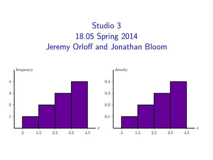
x frequency .5 1.5 2.5 3.5 4.5 1 2 3 4 x density .5 1.5 2.5 3.5 4.5 0.1 0.2 0.3 0.4
Studio 3 18.05 Spring 2014 Jeremy Orloff and Jonathan Bloom - - PowerPoint PPT Presentation
Studio 3 18.05 Spring 2014 Jeremy Orloff and Jonathan Bloom frequency density 4 0.4 3 0.3 2 0.2 1 0.1 x x .5 1.5 2.5 3.5 4.5 .5 1.5 2.5 3.5 4.5 Concept questions Suppose X is a continuous random variable. a) What is P ( a X
x frequency .5 1.5 2.5 3.5 4.5 1 2 3 4 x density .5 1.5 2.5 3.5 4.5 0.1 0.2 0.3 0.4
July 13, 2014 2 / 10
July 13, 2014 3 / 10
July 13, 2014 4 / 10
July 13, 2014 5 / 10
July 13, 2014 6 / 10
July 13, 2014 7 / 10
July 13, 2014 8 / 10
x frequency .5 1.5 2.5 3.5 4.5 1 2 3 4 x density .5 1.5 2.5 3.5 4.5 0.1 0.2 0.3 0.4
July 13, 2014 9 / 10
July 13, 2014 10 / 10
MIT OpenCourseWare http://ocw.mit.edu
Spring 201 For information about citing these materials or our Terms of Use, visit: http://ocw.mit.edu/terms.