
SLIDE 1
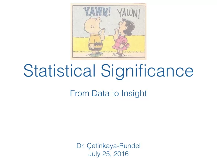
Statistical Significance
From Data to Insight
- Dr. Çetinkaya-Rundel
July 25, 2016
Statistical Significance From Data to Insight Dr. etinkaya-Rundel - - PowerPoint PPT Presentation
Statistical Significance From Data to Insight Dr. etinkaya-Rundel July 25, 2016 Is yawning contagious? 2 Do you think yawning is contagious? (A) Yes (B) No 3 Is yawning contagious? http://www.discovery.com/tv-shows/mythbusters/
July 25, 2016
2
(A) Yes (B) No
3
http://www.discovery.com/tv-shows/mythbusters/ videos/is-yawning-contagious-minimyth.htm
4
5
Treatment Control Total Yawn 10 4 14 Not yawn 24 12 36 Total 34 16 50 % yawners
0.29 0.25
Yawning and seeing someone yawn are independent
dependent
6
happened by chance if the null hypothesis were true?”
7
question, i.e. what we’re testing for
hypothesis is true, either via simulation or theoretical methods
convincing evidence for the alternative hypothesis, stick with the null hypothesis
alternative
8
2-10, 4 jacks, 4 queens, and 4 kings.
study:
yawn.
9
DEMO: Watch me go through the activity before you start it in your teams
are from a random process
and submit this value using your clicker (value must be between 0 and 1) -
10
11
0.2 0.4
the difference between the proportions of yawners in the treatment and control groups was due to chance (yawning and seeing someone yawn are independent)
data → the difference between the proportions of yawners in the treatment and control groups was not due to chance (yawning and seeing someone yawn are dependent)
12
Do the simulation results suggest that yawning is contagious, i.e. does seeing someone yawn and yawning appear to be dependent? (Hint: In the actual data the difference was 0.04, does this appear to be an unusual observation for the chance model?)
(A) Yes (B) No
13
hypothesis
alternative:
alternative hypothesis
14
15
students were asked to tap their fingers at a rapid rate.
10 students each.
coffee, which included about 200 mg of caffeine for the students in one group but was decaffeinated coffee for the second group.
measure finger tapping rate (taps per minute).
16
17
(A) Bar plot (B) Scatterplot (C) Pie chart (D) Side-by-side box plots (E) Single box plot
18
19
We are interested in finding out if caffeine increases tapping rate. Which of the following are the correct set of hypotheses? Note: μ = population mean, x = sample mean
(A) H0 : μcaff = μno caff; HA : μcaff < μno caff (B) H0 : μcaff = μno caff; HA : μcaff > μno caff (C) H0 : xcaff = xno caff; HA : xcaff > xno caff (D) H0 : μcaff > μno caff; HA : μcaff = μno caff (E) H0 : μcaff = μno caff; HA : μcaff ≠ μno caff
20
in the study.
cards each, label one stack “caffeine” and the other stack “no caffeine”.
groups, and record the difference on a dot plot.
randomization distribution.
21
Below is a randomization distribution of 100 simulated differences in means (xcaff - xno caff). Calculate the p-value for the hypothesis test evaluating whether caffeine increases average tapping rate.
22
difference between the medians instead of the means
simulations where the simulated difference in medians is at least 3.
23
Below is a randomization distribution of 100 simulated differences in medians (mediancaff - medianno caff). Calculate the p-value for the hypothesis test evaluating whether caffeine increases median tapping rate.
24