[PDF] - Statistical Natural Language Processing . ltekin, variables PDF Document

SLIDE 1

Statistical Natural Language Processing

Unsupervised machine learning Çağrı Çöltekin

University of Tübingen Seminar für Sprachwissenschaft

Summer Semester 2017

Recap Clustering PCA Autoencoders Practical matters

Supervised learning

The methods we studied so far are instances of supervised

learning

In supervised learning, we have a set of predictors x, and

want to predict a response or outcome variable y

During training, we have both input and output variables
Training consist of estimating parameters w of a model
During prediction, we are given x and make predictions

based on model we learned

Ç. Çöltekin, SfS / University of Tübingen Summer Semester 2017 1 / 53 Recap Clustering PCA Autoencoders Practical matters

Supervised learning: regression

x y

The response (outcome)

variable (y) is a quantitative variable.

Given the features (x) we

want to predict the value

f y

Ç. Çöltekin, SfS / University of Tübingen Summer Semester 2017 2 / 53 Recap Clustering PCA Autoencoders Practical matters

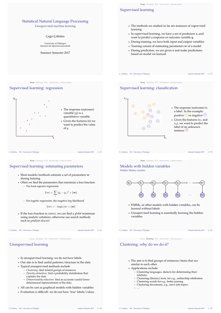
Supervised learning: classifjcation

x1 x2 + + + + + + − − − − − − − ?

The response (outcome) is

a label. In the example: positive + or negative −

Given the features (x1 and

x2), we want to predict the label of an unknown instance ?

Ç. Çöltekin, SfS / University of Tübingen Summer Semester 2017 3 / 53 Recap Clustering PCA Autoencoders Practical matters

Supervised learning: estimating parameters

Most models/methods estimate a set of parameters w

during training

Often we fjnd the parameters that minimize a loss function

– For least-squares regression J(w) = ∑

i

(ˆ yi − yi)2 + ∥w∥ – For logistic regression, the negative log likelihood J(w) = −logL(w) + ∥w∥

If the loss function is convex, we can fjnd a global minimum

using analytic solutions, otherwise use search methods such as gradient descent

Ç. Çöltekin, SfS / University of Tübingen Summer Semester 2017 4 / 53 Recap Clustering PCA Autoencoders Practical matters

Models with hidden variables

Hidden Markov models

q0 q1 q2 q3 q4 … qT

1
2
3
4

…

T
HMMs, or other models with hidden variables, can be

learned without labels

Unsupervised learning is essentially learning the hidden

variables

Ç. Çöltekin, SfS / University of Tübingen Summer Semester 2017 5 / 53 Recap Clustering PCA Autoencoders Practical matters

Unsupervised learning

In unsupervised learning, we do not have labels
Our aim is to fjnd useful patterns/structure in the data
Typical unsupervised methods include

– Clustering: fjnd related groups of instances – Density estimation: fjnd a probability distribution that explains the data – Dimensionality reduction: fjnd an accurate/useful lower dimensional representation of the data

All can be cast as graphical models with hidden variables
Evaluation is diffjcult: we do not have ‘true’ labels/values

Ç. Çöltekin, SfS / University of Tübingen Summer Semester 2017 6 / 53 Recap Clustering PCA Autoencoders Practical matters

Clustering: why do we do it?

The aim is to fjnd groups of instances/items that are

similar to each other

Applications include

– Clustering languages, dialects for determining their relations – Clustering (literary) texts, for e.g., authorship attribution – Clustering words for e.g., better parsing – Clustering documents, e.g., news into topics – …

Ç. Çöltekin, SfS / University of Tübingen Summer Semester 2017 7 / 53

SLIDE 2

Recap Clustering PCA Autoencoders Practical matters

Clustering

Clustering can be hierarchical or non-hierarchical
Clustering can be bottom-up (agglomerative) or top-down

(divisive)

For most (useful) problems we cannot fjnd globally
ptimum solutions, we often rely on greedy algorithms

that fjnd a local minimum

The measure of distance or similarity between the items is

important

Ç. Çöltekin, SfS / University of Tübingen Summer Semester 2017 8 / 53 Recap Clustering PCA Autoencoders Practical matters

Clustering in two dimensional space

x1 x2

Unlike classifjcation, we do

not have labels

We want to fjnd ‘natural’

groups in the data

Intuitively, similar or

closer data points are grouped together

Ç. Çöltekin, SfS / University of Tübingen Summer Semester 2017 9 / 53 Recap Clustering PCA Autoencoders Practical matters

Similarity and distance

The notion of distance (similarity) is important in
clustering. A distance measure D,

– is symmetric: D(a, b) = D(b, a) – non-negative: D(a, b) ⩾ 0 for all a, b, and it D(a, b) = 0 ifg a = b – obeys triangle inequality: D(a, b) + D(b, c) ⩾ D(a, c)

The choice of distance is application specifjc
We will often face with defjning distance measures

between linguistic units (letters, words, sentences, documents, …)

Ç. Çöltekin, SfS / University of Tübingen Summer Semester 2017 10 / 53 Recap Clustering PCA Autoencoders Practical matters

Distance measures in Euclidean space

Euclidean distance:

∥a − b∥ =

k

∑

j=1

(aj − bj)2

Manhattan distance:

∥a − b∥1 =

k

∑

j=1

|aj − bj|

Ç. Çöltekin, SfS / University of Tübingen Summer Semester 2017 11 / 53 Recap Clustering PCA Autoencoders Practical matters

How to do clustering

Most clustering algorithms try to minimize the scatter within each cluster. Which is equivalent to maximizing the scatter between clusters x1 x2

K

∑

k=1

∑

C(a)=k

∑

C(b)=k

d(a, b)

K

∑

k=1

∑

C(a)=k

∑

C(b)̸=k

d(a, b)

Ç. Çöltekin, SfS / University of Tübingen Summer Semester 2017 12 / 53 Recap Clustering PCA Autoencoders Practical matters

K-means clustering

K-means is a popular method for clustering.

1. Randomly choose centroids, m1, . . . , mK, representing K

clusters

2. Repeat until convergence

– Assign each data point to the cluster of the nearest centroid – Re-calculate the centroid locations based on the assignments

Efgectively, we are fjnding a local minimum of the sum of squared Euclidean distance within each cluster 1 2

K

∑

k=1

∑

C(a)=k

∑

C(b)=k

∥a − b∥2

* Note the similarity with the EM algorithm

Ç. Çöltekin, SfS / University of Tübingen Summer Semester 2017 13 / 53 Recap Clustering PCA Autoencoders Practical matters

K-means clustering: visualization

1 2 3 4 5 1 2 3 4 5

The data
Set cluster centroids

randomly

Assign data points

to the closest centroid

Recalculate the

centroids

Ç. Çöltekin, SfS / University of Tübingen Summer Semester 2017 14 / 53 Recap Clustering PCA Autoencoders Practical matters

K-means clustering: visualization

1 2 3 4 5 1 2 3 4 5

The data
Set cluster centroids

randomly

Assign data points

to the closest centroid

Recalculate the

centroids

Ç. Çöltekin, SfS / University of Tübingen Summer Semester 2017 14 / 53

SLIDE 3

Recap Clustering PCA Autoencoders Practical matters

K-means clustering: visualization

1 2 3 4 5 1 2 3 4 5

The data
Set cluster centroids

randomly

Assign data points

to the closest centroid

Recalculate the

centroids

Ç. Çöltekin, SfS / University of Tübingen Summer Semester 2017 14 / 53 Recap Clustering PCA Autoencoders Practical matters

K-means clustering: visualization

1 2 3 4 5 1 2 3 4 5

The data
Set cluster centroids

randomly

Assign data points

to the closest centroid

Recalculate the

centroids

Ç. Çöltekin, SfS / University of Tübingen Summer Semester 2017 14 / 53 Recap Clustering PCA Autoencoders Practical matters

K-means clustering: visualization

1 2 3 4 5 1 2 3 4 5

The data
Set cluster centroids

randomly

Assign data points

to the closest centroid

Recalculate the

centroids

Ç. Çöltekin, SfS / University of Tübingen Summer Semester 2017 14 / 53 Recap Clustering PCA Autoencoders Practical matters

K-means clustering: visualization

1 2 3 4 5 1 2 3 4 5

The data
Set cluster centroids

randomly

Assign data points

to the closest centroid

Recalculate the

centroids

Ç. Çöltekin, SfS / University of Tübingen Summer Semester 2017 14 / 53 Recap Clustering PCA Autoencoders Practical matters

K-means clustering: visualization

1 2 3 4 5 1 2 3 4 5

The data
Set cluster centroids

randomly

Assign data points

to the closest centroid

Recalculate the

centroids

Ç. Çöltekin, SfS / University of Tübingen Summer Semester 2017 14 / 53 Recap Clustering PCA Autoencoders Practical matters

K-means clustering: visualization

1 2 3 4 5 1 2 3 4 5

The data
Set cluster centroids

randomly

Assign data points

to the closest centroid

Recalculate the

centroids

Ç. Çöltekin, SfS / University of Tübingen Summer Semester 2017 14 / 53 Recap Clustering PCA Autoencoders Practical matters

K-means: issues

K-means requires the data to be in an Euclidean space
K-means is sensitive to outliers
The results are sensitive to initialization

– There are some smarter ways to select initial points – One can do multiple initializations, and pick the best (with lowest within-group squares)

It works well with approximately equal-size round-shaped

clusters

We need to specify number of clusters in advance

Ç. Çöltekin, SfS / University of Tübingen Summer Semester 2017 15 / 53 Recap Clustering PCA Autoencoders Practical matters

How many clusters?

The number of clusters is defjned for some problems, e.g.,

classifying news into a fjxed set of topics/interests

For others, there is no clear way to select the best number
f clusters
The error (within cluster scatter) always decreases with

increasing number of clusters, using a test set or cross validation is not useful either

A common approach is clustering for multiple K values,

and picking where there is an ‘elbow’ in the graph against the error function

Ç. Çöltekin, SfS / University of Tübingen Summer Semester 2017 16 / 53

SLIDE 4

Recap Clustering PCA Autoencoders Practical matters

How many clusters?

K J(w)

1 2 3 4 5 6 7 8 9 40 80 120 160

This plot is sometimes called a scree plot.

Ç. Çöltekin, SfS / University of Tübingen Summer Semester 2017 17 / 53 Recap Clustering PCA Autoencoders Practical matters

K-medoids

K-medoids algorithm is an alternation of K-means
Instead of calculating centroids, we try to fjnd most typical

data point at each iteration

K-medoids can work with distances, does not need feature

vectors to be in an Euclidean space

It is less sensitive to outliers
It is computationally more expensive than K-means

Ç. Çöltekin, SfS / University of Tübingen Summer Semester 2017 18 / 53 Recap Clustering PCA Autoencoders Practical matters

Density estimation

K-means treats all data points in a cluster equally
A ‘soft’ version of K-means is density estimation for

Gaussian mixtures, where

– We assume the data comes from a mixture of K Gaussian distributions – We try to fjnd the parameters of each distribution (instead

f centroids) that maximizes the likelihood of the data
Unlike K-means, mixture of Gaussians assigns probabilities

for each data point belonging to one of the clusters

It is typically estimated using the

expectation-maximization (EM) algorithm

Ç. Çöltekin, SfS / University of Tübingen Summer Semester 2017 19 / 53 Recap Clustering PCA Autoencoders Practical matters

Density estimation using the EM algorithm

The EM algorithm (or its variations) is used in learning

models with latent/hidden variables

It is closely related to the K-means algorithm
1. Initialize the parameters (e.g., randomly) of K multivariate

normal distributions (µ, Σ)

2. Iterate until convergence:

E-step Given the parameters, compute the membership ‘weights’, the probability of each data point belonging to each distribution M-step Re-estimate the mixture density parameters using the calculated membership weights in the E-step

Ç. Çöltekin, SfS / University of Tübingen Summer Semester 2017 20 / 53 Recap Clustering PCA Autoencoders Practical matters

Hierarchical clustering

Instead of fmat division to clusters as in K-means,

hierarchical clustering builds a hierarchy based on similarity of the data points

There are two main ‘modes of operation’:

Bottom-up or agglomerative clustering

starts with individual data points,
merges the clusters until all data is in a single cluster

Top-down or divisive clustering

starts with a single cluster,
and splits until all leaves are single data points

Ç. Çöltekin, SfS / University of Tübingen Summer Semester 2017 21 / 53 Recap Clustering PCA Autoencoders Practical matters

Hierarchical clustering

Hierarchical clustering operates on difgerences
The result is a binary tree called dendrogram
Dendrograms are easy to interpret (especially if data is

hierarchical)

The algorithm does not commit to the number of clusters K

from the start, the dendrogram can be ‘cut’ at any height for for determining the clusters

Ç. Çöltekin, SfS / University of Tübingen Summer Semester 2017 22 / 53 Recap Clustering PCA Autoencoders Practical matters

Agglomerative clustering

1. Compute the

similarity/distance matrix

2. Assign each data point to

its own cluster

3. Repeat until no clusters left

to merge

– Pick two clusters that are most similar to each

ther

– Merge them into a single cluster

1 2 3 4 5

Ç. Çöltekin, SfS / University of Tübingen Summer Semester 2017 23 / 53 Recap Clustering PCA Autoencoders Practical matters

Agglomerative clustering demonstration

1 2 3 4 5 x1 x2 1 2 3 4 5

Ç. Çöltekin, SfS / University of Tübingen Summer Semester 2017 24 / 53

SLIDE 5

Recap Clustering PCA Autoencoders Practical matters

How to calculate between cluster distances

Complete maximal inter-cluster distance Single minimal inter-cluster distance Average mean inter-cluster distance Centroid distance between the centroids x1 x2 1 2 3 4 5

Note: we only need distances, (feature) vectors are not necessary

Ç. Çöltekin, SfS / University of Tübingen Summer Semester 2017 25 / 53 Recap Clustering PCA Autoencoders Practical matters

How to calculate between cluster distances

Complete maximal inter-cluster distance Single minimal inter-cluster distance Average mean inter-cluster distance Centroid distance between the centroids x1 x2 1 2 3 4 5

Note: we only need distances, (feature) vectors are not necessary

Ç. Çöltekin, SfS / University of Tübingen Summer Semester 2017 25 / 53 Recap Clustering PCA Autoencoders Practical matters

How to calculate between cluster distances

Complete maximal inter-cluster distance Single minimal inter-cluster distance Average mean inter-cluster distance Centroid distance between the centroids x1 x2 1 2 3 4 5

Note: we only need distances, (feature) vectors are not necessary

Ç. Çöltekin, SfS / University of Tübingen Summer Semester 2017 25 / 53 Recap Clustering PCA Autoencoders Practical matters

How to calculate between cluster distances

Complete maximal inter-cluster distance Single minimal inter-cluster distance Average mean inter-cluster distance Centroid distance between the centroids x1 x2 1 2 3 4 5

Note: we only need distances, (feature) vectors are not necessary

Ç. Çöltekin, SfS / University of Tübingen Summer Semester 2017 25 / 53 Recap Clustering PCA Autoencoders Practical matters

Clustering: some closing notes

We do not have proper evaluation procedures for

clustering results (for unsupervised learning in general)

Clustering is typically unstable, slight changes in the data
r parameter choices may change the results drastically
Approaches against instability include some validation

methods, or producing ‘probabilistic’ dendrograms by running clustering with difgerent options

Ç. Çöltekin, SfS / University of Tübingen Summer Semester 2017 26 / 53 Recap Clustering PCA Autoencoders Practical matters

Principal component Analysis

Principal component analysis (PCA) is a method of

dimensionality reduction

PCA maps the original data into a lower dimensional space

by a linear transformation (rotation)

The transformed variables retain most of the variation

(=information) in the input

PCA can be used for

– visualization – data compression – reducing dimensionality for use in supervised methods – eliminating noise

Ç. Çöltekin, SfS / University of Tübingen Summer Semester 2017 27 / 53 Recap Clustering PCA Autoencoders Practical matters

PCA: a toy example

x1 x2

p1 p2 p3

4
4
3
3
2
2
1
1

1 1 2 2 3 3 4 4

Questions:

How many dimensions do

we have?

How many dimensions do

we need?

Short divergence: calculate

the covariance matrix Σ = [ 18

3

8 8

32 3

]

Ç. Çöltekin, SfS / University of Tübingen Summer Semester 2017 28 / 53 Recap Clustering PCA Autoencoders Practical matters

PCA: A toy example (2)

x1 x2

p1 p2 p3

4
4
3
3
2
2
1
1

1 1 2 2 3 3 4 4

What if we reduce the data to: z1 z2

p1 p2 p3

5

5

Going back to the original coordinates is easy, rotate using: A = [cos θ − sin θ sin θ cos θ ] = [ 3

5

− 4

5 4 5 3 5

] p1 = A× [−5 ] = [−3 −4 ] p1 = A× [0 ] = [0 ] p1 = A× [5 ] = [3 4 ] We can recover the original points perfectly. In this example the inherent dimensionality of the data is only 1.

Ç. Çöltekin, SfS / University of Tübingen Summer Semester 2017 29 / 53

SLIDE 6

Recap Clustering PCA Autoencoders Practical matters

PCA: A toy example (3)

x1 x2

p1 p2 p3

4
4
3
3
2
2
1
1

1 1 2 2 3 3 4 4

What if the variables were

not perfectly but strongly correlated?

We could still do a similar

transformation:

z1 z2

p1 p2 p3

5

5

Discarding z2 results in a

small reconstruction error: p1 = A × [−5 ] = [−3 −4 ]

Note: z1 (also z2) is a linear

combination of original variables

Ç. Çöltekin, SfS / University of Tübingen Summer Semester 2017 30 / 53 Recap Clustering PCA Autoencoders Practical matters

Why do we want to reduce the dimensionality

Visualizing high-dimensional data becomes possible
If we use the data for supervised learning, we avoid ‘the

curse of dimensionality’

Decorrelation is useful in some applications
We compress the data (in a lossy way)
We eliminate noise (assuming a high signal to noise ratio)

Ç. Çöltekin, SfS / University of Tübingen Summer Semester 2017 31 / 53 Recap Clustering PCA Autoencoders Practical matters

Difgerent views on PCA

x1 x2 PC1

Find the direction of the

largest variance

Find the projection with

the least reconstruction error

Find a lower dimensional

latent Gaussian variable such that the observed variable is a mapping of the latent variable to a higher dimensional space (with added noise)

Ç. Çöltekin, SfS / University of Tübingen Summer Semester 2017 32 / 53 Recap Clustering PCA Autoencoders Practical matters

How to fjnd PCs

When viewed as maximizing variance or reducing the re

construction error, we can write the appropriate objective function and fjnd the vectors that minimize it

In latent variable interpretation, we can use EM as in

estimating mixtures of Gaussians

The principle components are the eigenvectors of the

correlation matrix, where large eigenvalues correspond to components with large variation

A numerically stable way to obtain principal components is

doing singular value decomposition (SVD) on the input data

Ç. Çöltekin, SfS / University of Tübingen Summer Semester 2017 33 / 53 Recap Clustering PCA Autoencoders Practical matters

PCA as matrix factorization (eigenvalue decomposition)

One can compute PCA by decomposing the covariance

matrix as (note Σ = XTX) Σ = UΛUT

– the columns of U are the principal components (eigenvectors) – Λ is a diagonal matrix of eigenvalues

Another option is SVD, which factorizes the input vector

(k variables × n data points) as X = UDV∗

– U (k × k) contains the eigenvectors as before, – D (k × k) diagonal matrix D2 = Λ – V∗ is a k × n unitary matrix

* The above is correct for standardized variables, otherwise the formulas get slightly more complicated. Ç. Çöltekin, SfS / University of Tübingen Summer Semester 2017 34 / 53 Recap Clustering PCA Autoencoders Practical matters

A practical example

(with simplifjed/fake data)

Our data consists of ‘measurements’ from speech signal of

instances of two vowels, we have 12 measurements for each vowel instance

        5.19 4.33 14.76 30.08 14.73 7.06 15.56 24.46 8.51 . . . 2.99 5.25 11.69 19.27 18.02 11.04 13.34 38.13 8.70 . . . 6.25 6.05 13.88 19.26 17.81 6.95 12.58 39.74 9.58 . . . 7.24 5.43 15.15 18.93 15.69 10.18 14.89 34.86 10.03 . . . 6.07 6.27 13.34 17.60 19.98 11.04 13.28 36.02 8.66 . . . . . .        

How do we visualize this data?
Are all 12 variables useful?

Ç. Çöltekin, SfS / University of Tübingen Summer Semester 2017 35 / 53 Recap Clustering PCA Autoencoders Practical matters

A practical example

Visualizing with pairwise scatter plots

V1

2 4 6 8 10 15 20 25 2 4 6 8 2 4 6 8 10

V2 V3

10 14 18 2 3 4 5 6 7 8 9 15 20 25 10 12 14 16 18

V4

…

Ç. Çöltekin, SfS / University of Tübingen Summer Semester 2017 36 / 53 Recap Clustering PCA Autoencoders Practical matters

A practical example

Plotting the fjrst two principal components

10
5

5 10

5

5 PC1 PC2

Ç. Çöltekin, SfS / University of Tübingen Summer Semester 2017 37 / 53

SLIDE 7

Recap Clustering PCA Autoencoders Practical matters

A practical example

How many components to keep? (scree plot)

Variances 10 20 30 40 50 60 1 2 3 4 5 6 7 8 9 10

Ç. Çöltekin, SfS / University of Tübingen Summer Semester 2017 38 / 53 Recap Clustering PCA Autoencoders Practical matters

Some practical notes on PCA

Variables need to be centered
Scales of the variables matter, standardizing may be a good

idea depending on the units/scales of the individual variables

The sign of the principal component (vector) is not

important

If there are more variables than the data points, we can still

calculate the principal components, but there will be at most n − 1 PCs

PCA will be successful if variables are linearly correlated,

there are extensions for dealing with nonlinearities (e.g., kernel PCA, ICA)

Ç. Çöltekin, SfS / University of Tübingen Summer Semester 2017 39 / 53 Recap Clustering PCA Autoencoders Practical matters

Unsupervised learning: a summary (so far)

In unsupervised learning, we do not have labels. Our aim

is to fjnd/exploit (latent) structure in the data

We studied a number of related methods

Clustering fjnds groups in the data Mixture densities are a ‘soft’ version of the clustering, assuming data is generated by a number of distributions Dimensionality reduction methods try to summarize the data with fewer variables/dimensions

The evaluation of unsupervised methods are problematic,

without knowing what we should exactly fjnd in the data

Ç. Çöltekin, SfS / University of Tübingen Summer Semester 2017 40 / 53 Recap Clustering PCA Autoencoders Practical matters

Unsupervised learning in ANNs

Restricted Boltzmann machines (RBM)

similar to the latent variable models (e.g., Gaussian mixtures), consider the representation learned by hidden layers as hidden variables (h), and learn p(x, h) that maximize the probability of the (unlabeled)data

Autoencoders

train a constrained feed-forward network to predict its

utput

Ç. Çöltekin, SfS / University of Tübingen Summer Semester 2017 41 / 53 Recap Clustering PCA Autoencoders Practical matters

Restricted Boltzmann machines (RBMs)

x1 h1 x2 h2 x3 h3 x4 h4 W h x

RBMs are unsupervised latent

variable models, they learn only from unlabeled data

They are generative models of

the joint probability p(h, x)

They correspond to undirected

graphical models

No links within layers
The aim is to learn useful

features (h)

*Biases are omitted in the diagrams and the formulas for simplicity. Ç. Çöltekin, SfS / University of Tübingen Summer Semester 2017 42 / 53 Recap Clustering PCA Autoencoders Practical matters

The distribution defjned by RBMs

x1 h1 x2 h2 x3 h3 x4 h4 W p(h, x) = ehT Wx Z This calculation is intractable (Z is diffjcult to calculate). But conditional distributions are easy to calculate p(h|x) = ∏

j

p(hj|x) = 1 1 + eWjx p(x|h) = ∏

k

p(xk|h) = 1 1 + eWT

kh Ç. Çöltekin, SfS / University of Tübingen Summer Semester 2017 43 / 53 Recap Clustering PCA Autoencoders Practical matters

Learning in RBMs

We want to maximize the probability the model assigns to

the input, p(x), or equivalently minimize − log p(x)

In general, this is computationally expensive
Contrastive divergence algorithm is a well known algorithm

that effjciently fjnds an approximate solution

Ç. Çöltekin, SfS / University of Tübingen Summer Semester 2017 44 / 53 Recap Clustering PCA Autoencoders Practical matters

Autoencoders

x1 ˆ x1 x2 ˆ x2 h1 x3 ˆ x3 h2 x4 ˆ x4 h3 x5 ˆ x5 W W∗

Encoder Decoder

Autoencoders are standard

feed-forward networks

The main difgerence is that

they are trained to predict their input (they try to learn the identity function)

The aim is to learn useful

representations of input at the hidden layer

Typically weights are tied

(W∗ = WT)

Ç. Çöltekin, SfS / University of Tübingen Summer Semester 2017 45 / 53

SLIDE 8

Recap Clustering PCA Autoencoders Practical matters

Under-complete autoencoders

x1 ˆ x1 x2 ˆ x2 h1 x3 ˆ x3 h2 x4 ˆ x4 h3 x5 ˆ x5

An autoencoder is said to be

under-complete if there are fewer hidden units than inputs

The network is forced to learn

a compact representation of the input (compress)

An autoencoder with a single

hidden layer is equivalent to PCA

We need multiple layers for

learning non-linear features

Ç. Çöltekin, SfS / University of Tübingen Summer Semester 2017 46 / 53 Recap Clustering PCA Autoencoders Practical matters

Over-complete autoencoders

h1 h2 x1 ˆ x1 h3 x2 ˆ x2 h4 x3 ˆ x3 h5

An autoencoder is said to be
ver-complete if there are more

hidden units than inputs

The network can normally

memorize the input perfectly

This type of networks are

useful if trained with a regularization term resulting in sparse hidden units (e.g., L1 regularization)

Ç. Çöltekin, SfS / University of Tübingen Summer Semester 2017 47 / 53 Recap Clustering PCA Autoencoders Practical matters

Denoising autoencoders

x1 ˆ x1 x2 x2 ˆ x2 h1 x3 ˆ x3 h2 x4 x4 ˆ x4 h3 x5 x5 ˆ x5 x

x

h ˆ x

Instead of providing the exact

input, we introduce noise by

– randomly setting some inputs to 0 (dropout) – adding random (Gaussian) noise

Network is still expected to

reconstruct the original input (without noise)

Ç. Çöltekin, SfS / University of Tübingen Summer Semester 2017 48 / 53 Recap Clustering PCA Autoencoders Practical matters

Unsupervised pre-training

A common use case for RBMs and autoencoders are as

pre-training methods for supervised networks

Autoencoders or RBMs are trained using unlabeled data
The weights learned during the unsupervised learning is

used for initializing the weights of a supervised network

This approach has been one of the reasons for success of

deep networks

Ç. Çöltekin, SfS / University of Tübingen Summer Semester 2017 49 / 53 Recap Clustering PCA Autoencoders Practical matters

Deep unsupervised learning

Both autoencoders and RBMs can be ‘stacked’
Learn the weights of the fjrst hidden layer from the data
Freeze the weights, and using the hidden layer activations

as input, train another hidden layer, …

This approach is called greedy layer-wise training
In case of RBMs resulting networks are called deep belief

networks

Deep autoencoders are called stacked autoencoders

Ç. Çöltekin, SfS / University of Tübingen Summer Semester 2017 50 / 53 Recap Clustering PCA Autoencoders Practical matters

Summary

Unsupervised methods try to discover ‘hidden’ structure

in the data

Clustering is used for fjnding groups of clusters in the data

without labels

Dimensionality reduction transforms the data in a low

dimensional space while keeping most of the information in the original data

RBM and autoencoders learn (typically lover dimensional,

dense, continuous) representations of the input that are useful in other tasks Next: Today(?) Distributed representations Wed(?) Text classifjcation

Ç. Çöltekin, SfS / University of Tübingen Summer Semester 2017 51 / 53 Recap Clustering PCA Autoencoders Practical matters

Exam

On Wednesday July 26
It should take about an hour
Mix of true/false questions and long-answer questions
Your main source is the course slides, the recommended

reading will help

Understanding the graded/ungraded exercises is

important

Focus will be on NLP methods/applications
Questions measuring your understanding of the

methods/topics, no emphasis on memorizing

You can bring an A4 cheat sheet, both sides are OK, should

be readable to the unaided eye

Ç. Çöltekin, SfS / University of Tübingen Summer Semester 2017 52 / 53 Recap Clustering PCA Autoencoders Practical matters

Last two graded assignments

Assignment 2 is posted today
Two deadlines

Jul 31 you get 1 point bonus, detailed feedback, an initial attempt may be helpful for the exam Oct 2 Full grade, but no feedback

Assignment 3 will be posted next week

– Topic will be sentiment analysis – Similar two-deadline schedule

Ç. Çöltekin, SfS / University of Tübingen Summer Semester 2017 53 / 53

SLIDE 9

Derivation of PCA by maximizing the variance

We focus on the fjrst PC (z1), which maximizes the

variance of the data onto itself

We are interested only on the direction, so we choose z1 to

be a unit vector (∥z1∥ = 1)

Remember that to project a vector onto another, we simply

use dot product, So the projected data points are zxi for i = 1, . . . , N.

The variance of the projected data points (that we want to

maximize) is, σz1 = 1 N

N

∑

i

(z1xi − z1¯ xi)2 = zT

1Σz

where Σx is the covariance matrix of the unprojected data

Ç. Çöltekin, SfS / University of Tübingen Summer Semester 2017 A.1

Derivation of PCA by maximizing the variance (cont.)

The problem becomes maximize

zT

1Σz

with the constraint ∥z1∥ = zT

1z1 = 1

Turning it into a unconstrained optimization problem with

Lagrange multipliers, we minimize zT

1Σz + λ1(1 − zT 1z1)

Taking the derivative and setting it to 0 gives us

Σz1 = λ1z1 Note: by defjnition, z1 is an eigenvector of Σ, and λ1 is the corresponding eigenvalue

z1 is the fjrst principal component, we can now compute

the second principal component with the constraint that it has to be orthogonal to the fjrst one

Ç. Çöltekin, SfS / University of Tübingen Summer Semester 2017 A.2