Sensitivity Analysis and Active Subspace Construction for Surrogate - PowerPoint PPT Presentation

Sensitivity Analysis and Active Subspace Construction for Surrogate Models Employed for Bayesian Inference Ralph C. 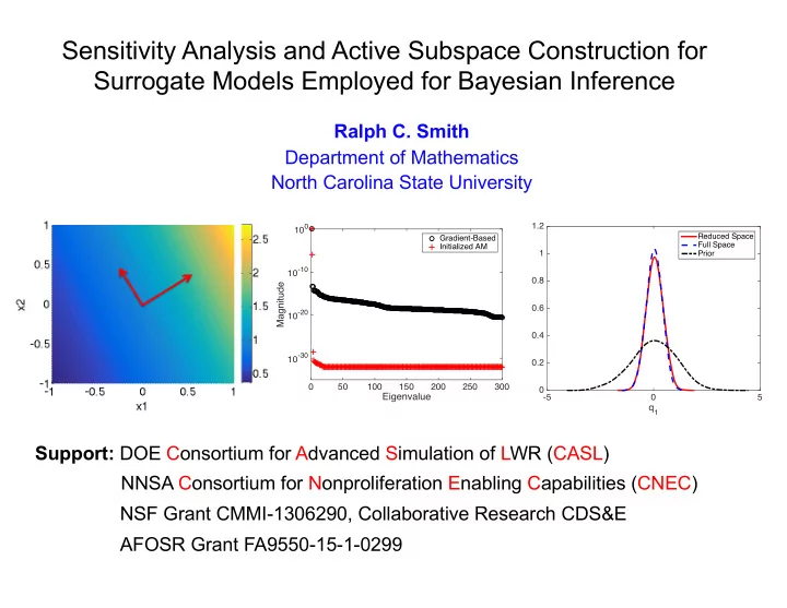Smith Department of Mathematics North Carolina State University 1.2 10 0 Reduced Space Gradient-Based Full Space Initialized AM 1 Prior 10 -10 0.8 Magnitude 0.6 10 -20 0.4 10 -30 0.2 0 50 100 150 200 250 300 0 Eigenvalue -5 0 5 q 1 Support: DOE Consortium for Advanced Simulation of LWR (CASL) NNSA Consortium for Nonproliferation Enabling Capabilities (CNEC) NSF Grant CMMI-1306290, Collaborative Research CDS&E AFOSR Grant FA9550-15-1-0299

Sensitivity Analysis and Active Subspace Construction for Surrogate Models Employed for Bayesian Inference Ralph C. Smith Department of Mathematics North Carolina State University 1.2 10 0 Reduced Space Gradient-Based Full Space Initialized AM 1 Prior 10 -10 0.8 Magnitude 0.6 10 -20 0.4 10 -30 0.2 0 50 100 150 200 250 300 0 Eigenvalue -5 0 5 q 1 ”We”: Kayla Coleman, Lider Leon, Allison Lewis, Mohammad Abdo (NCSU) Brian Williams (LANL), Max Morris (Iowa State University) Billy Oates, Paul Miles (Florida State University)

Example 1: Pressurized Water Reactors (PWR) Models: • Involve neutron transport, thermal-hydraulics, chemistry, fuels • Inherently multi-scale, multi-physics. Objective: Develop Virtual Environment for Reactor Applications (VERA)

Motivation for Active Subspace Construction 3-D Neutron Transport Equations: ∂ϕ 1 ∂ t + Ω · r ϕ + Σ t ( r , E ) ϕ ( r , E , Ω , t ) | v | Z Z 1 dE 0 Σ s ( E 0 ! E , Ω 0 ! Ω ) ϕ ( r , E 0 , Ω 0 , t ) d Ω 0 = 4 π 0 Z Z 1 + χ ( E ) d Ω 0 dE 0 ν ( E 0 ) Σ f ( E 0 ) ϕ ( r , E 0 , Ω 0 , t ) 4 π 4 π 0 Challenges: • Linear in the state but function of 7 independent variables: r = x , y , z ; E ; Ω = θ , φ ; t • Very large number of inputs; e.g., 100,000; Active subspace construction critical. • ORNL Code SCALE: can take minutes to hours to run. • SCALE TRITON has adjoint capabilities via TSUNAMI-2D and NEWT.

SCALE6.1: High-Dimensional Example Setup: Cross-section computations SCALE6.1 • Input Dimension: 7700 k eff • Output : Magnitude governs reactions Materials Reactions 234 10 31 92 U 5 B 15 P Σ t n Ñ γ 235 11 55 92 U 5 B 25 Mn Σ e n Ñ p 236 14 92 U 7 N 26 Fe n Ñ d Σ f 238 15 116 92 U 7 N 50 Sn Σ c n Ñ t 6 ss-304 - bpr clad 5 air in bprs 1 23 120 n Ñ 3 He 1 H 11 Na 50 Sn ¯ 4 borosilicate glass ν 3 water 2 cladding 1 2.561 wt % enriched fuel 16 27 8 O 13 Al 40 Zr n Ñ α χ 7 rod n-9 ! PWR Quarter Fuel Lattice 6 C 14 Si 19 K n Ñ n 1 n Ñ 2 n Note: • Requires determination of active subspace to reduce input dimensions. • Finite-difference approximations of gradient ineffective due to dimension

Motivation for Inference on Active Subspaces Thermo-Hydraulic Equations: Mass, momentum and energy balance for fluid ∂ ∂ t ( α f ρ f ) + r · ( α f ρ f v f ) = − Γ Notes: • Similar relations for gas ∂ v f ∂ t + α f ρ f v f · r v f + r · σ R f + α f r · σ + α f r p f α f ρ f and bubbly phases • Reduced models must = − F R − F + Γ ( v f − v g ) / 2 + α f ρ f g conserve mass, ∂ momentum and energy ∂ t ( α f ρ f e f ) + r · ( α f ρ f e f v f + Th ) = ( T g − T f ) H + T f ∆ f − T g ( H − α g r · h ) + h · r T − Γ [ e f + T f ( s ∗ − s f )] ✓ ∂α f ◆ ∂ t + r · ( α f v f ) + Γ − p f ρ f Note: • CFD and sub-channel codes can have 15-30 closure relations and up to 75 parameters. • Codes and closure relations often ”borrowed” from other physical phenomena; e.g., single phase fluids, airflow over a car (CFD code STAR-CCM+) • Calibration is necessary and closure relations can conflict.

Example 2. Multiscale Model Development Example: PZT-Based Macro-Fiber Composites ρ ¨ u = r · σ + F r · D = 0 , D = ε 0 E + P r ⇥ E = 0 , E = − r ϕ P = d ( E , σ ) σ + χ σ E + P irr ( E , σ ) P α = d α σ + χ σ α E + P α R ε = s E σ + d ( E , σ ) E + ε irr ( E , σ ) ε α = s E α σ + d α E + ε α R Homogenized Energy Model (HEM) Continuum Energy Relations

Quantum-Informed Continuum Models Objectives: • Employ density function theory (DFT) to construct/calibrate continuum energy relations. Lead Titanate Zirconate (PZT) – e.g., Landau energy ψ ( P ) = α 1 P 2 + α 11 P 4 + α 111 P 6 DFT Electronic Structure Simulation a a a a o 130 c P a 0 Landau energy Cubic Tetragonal 0 o UQ and SA Issues: • Is 6 th order term required to accurately c a a a o characterize material behavior? − 90 P 0 a a P 0 • Note: Determines molecular structure Rhombohedral Orthorhombic

Quantum-Informed Continuum Models Objectives: • Employ density function theory (DFT) to construct/calibrate continuum energy relations. – e.g., Landau energy Lead Titanate Zirconate (PZT) ψ ( P ) = α 1 P 2 + α 11 P 4 + α 111 P 6 DFT Electronic Structure Simulation Landau energy Broad Objective: UQ and SA Issues: • Use UQ/SA to help bridge scales • Is 6 th order term required to accurately from quantum to system characterize material behavior? • Note: Determines molecular structure

Global Sensitivity Analysis: Analysis of Variance Sobol’ Representation: Y = f ( q ) p X X f ( q ) = f 0 + f i ( q i ) + f ij ( q i , q j ) + · · · + f 12 ··· p ( q 1 , ... , q p ) i = 1 i 6 i < j 6 p p X X = f 0 + f u ( q u ) i = 1 | u | = i where Z f 0 = f ( q ) ρ ( a ) dq = E [ f ( q )] Γ f i ( q i ) = E [ f ( q ) | q i ] − f 0 f ij ( q i , q j ) = E [ f ( q ) | q i , q j ] − f i ( q i ) − f j ( q j ) − f 0 Typical Assumption: q 1 , q 2 , ... , q p independent. Then Sobol’ Indices: Z f u ( q u ) f v ( q v ) ρ ( q ) dq = 0 for u 6 = v S u = var [ f u ( q u )] Γ X T u = S v , p var [ f ( q )] X X ) var [ f ( q )] = var [ f u ( q u )] v ⊆ u Note: Magnitude of S i , T i quantify i = 1 | u | = i contributions of q i to var [ f ( q )]

Global Sensitivity Analysis Example: Quantum-informed continuum model Question: Do we use 4 th or 6 th -order Landau energy? ψ ( P , q ) = α 1 P 2 + α 11 P 4 + α 111 P 6 Parameters: q = [ α 1 , α 11 , α 111 ] Global Sensitivity Analysis: α 1 α 11 α 111 S k 0.62 0.39 0.01 T k 0.66 0.38 0.06 µ ∗ 0.17 0.07 0.03 k Conclusion: α 111 insignificant and can be fixed

Global Sensitivity Analysis Example: Quantum-informed continuum model Question: Do we use 4 th or 6 th -order Landau energy? ψ ( P , q ) = α 1 P 2 + α 11 P 4 + α 111 P 6 Problem: We obtain different distributions Parameters: when we perform Bayesian inference with q = [ α 1 , α 11 , α 111 ] fixed non-influential parameters Global Sensitivity Analysis: 0.1 0.08 α 1 α 11 α 111 0.05 0.04 S k 0.62 0.39 0.01 0 0 T k 0.66 0.38 0.06 -420 -380 -340 650 750 850 α 1 α 11 µ ∗ 0.17 0.07 0.03 k 0.03 All α 1 , α 11 sampled Conclusion: 0.02 α 111 insignificant and can be fixed 0.01 0 0 75 150 α 111

Global Sensitivity Analysis Example: Quantum-informed continuum model Question: Do we use 4 th or 6 th -order Landau energy? ψ ( P , q ) = α 1 P 2 + α 11 P 4 + α 111 P 6 Problem: • Parameters correlated Parameters: • Cannot fix α 111 q = [ α 1 , α 11 , α 111 ] α 1 Global Sensitivity Analysis: α 11 α 1 α 11 α 111 S k 0.62 0.39 0.01 T k 0.66 0.38 0.06 µ ∗ 0.17 0.07 0.03 k α 11 Note: Must accommodate correlation 13

Global Sensitivity Analysis: Analysis of Variance Sobol’ Representation: p Pros: X X f ( q ) = f 0 + f u ( q u ) • Provides variance decomposition i = 1 | u | = i that is analogous to independent One Solution: Take variance to obtain case p X X Cons: var [ f ( q )] = cov [ f u ( q u ) , f ( q )] i = 1 | u | = i • Indices can be negative and difficult Sobol’ Indices: to interpret S u = cov [ f u ( q u ) , f ( q )] • Often difficult to determine underlying var [ f ( q )] distribution • Monte Carlo approximation often prohibitively expensive.

Global Sensitivity Analysis: Analysis of Variance Sobol’ Representation: p Pros: X X f ( q ) = f 0 + f u ( q u ) • Provides variance decomposition i = 1 | u | = i that is analogous to independent One Solution: Take variance to obtain case p X X Cons: var [ f ( q )] = cov [ f u ( q u ) , f ( q )] i = 1 | u | = i • Indices can be negative and difficult Sobol’ Indices: to interpret S u = cov [ f u ( q u ) , f ( q )] • Often difficult to determine underlying var [ f ( q )] distribution • Monte Carlo approximation often Alternative: Construct active subspaces prohibitively expensive. • Can accommodate parameter correlation • Often effective in high-dimensional space; e.g., p = 7700 for neutronics example Additional Goal: Use Bayesian analysis on active subspace to construct posterior densities for physical parameters.

Active Subspaces Note: • Functions may vary significantly in only a few directions • “Active” directions may be linear combination of inputs y = exp ( 0.7 q 1 + 0.3 q 2 ) Example: • Varies most in [0.7, 0.3] direction • No variation in orthogonal direction q 2 q 1

Active Subspaces Note: • Functions may vary significantly in only a few directions • “Active” directions may be linear combination of inputs y = exp ( 0.7 q 1 + 0.3 q 2 ) Example: • Varies most in [0.7, 0.3] direction • No variation in orthogonal direction q 2 A Bit of History: • Often attributed to Russi (2010). q 1