segmented regression model 11 oct 2014
play

Segmented Regression Model 11 Oct, 2014 1E 2014 NNN 1 1E 2014 - PDF document

Segmented Regression Model 11 Oct, 2014 1E 2014 NNN 1 1E 2014 NNN 2 Segmented Are Global Regression Models Temperatures Increasing Milo Schield 1 year averages Augsburg College Which source? Editor of www.StatLit.org US Rep:


  1. Segmented Regression Model 11 Oct, 2014 1E 2014 NNN 1 1E 2014 NNN 2 Segmented Are Global Regression Models Temperatures Increasing Milo Schield 1 year averages Augsburg College Which source? Editor of www.StatLit.org US Rep: International Statistical Literacy Project Surface or Fall 2014 satellite National Numeracy Network Conference based? www.StatLit.org/pdf/2014-Schield-NNN5-Slides.pdf 1E 2014 NNN 3 1E 2014 NNN 4 Are Global Surface Global Surface Temperatures: Temperatures Still Increasing Are they Still Increasing? Averaged over what time period? One-year or five? . Mean 5 year Temperature (C) Anomaly Base: 1951 ‐ 1990 Average Global Surface Temperatures (GISS): 0.65 Averages: 1 year vs 5 year 0.70 0.65 0.55 0.60 0.55 0.45 0.50 Slope: +1.6 C per 100 years Five ‐ year average: 0.45 R ‐ sq = 0.78 Two years on each side 0.40 0.35 One ‐ year average 0.35 http://data.giss.nasa.gov/gistemp/graphs_v3/ 0.30 0.25 0.25 1994 1996 1998 2000 2002 2004 2006 2008 2010 1994 1996 1998 2000 2002 2004 2006 2008 2010 2012 1E 2014 NNN 5 1E 2014 NNN 6 Minimize Total Error Using a Two-Segment Model Relative to Predicted . Least-squares regression works when data is nearly linear. Joint Std. Error in Y given X (STEYX) Rather than transform, consider a segmented linear model. 0.045 The goal is unchanged: minimum variation about model. 0.040 Best cutpoint of 0.035 two segments GISS Mean 5 year Temperature (C) Anomaly GISS Mean 5 year Temperature (C) Anomaly Cut Point: 1998 Cut Point: 2007 is at 2004 0.65 0.65 0.030 Base: 1951 ‐ 1990 Average 0.55 0.55 0.025 0.45 0.45 0.020 Joint STEYX is weighted average 0.35 of STEYX1 and STEYX2 0.35 Base: 1951 ‐ 0.015 1990 Average 0.25 0.25 1994 1996 1998 2000 2002 2004 2006 2008 2010 1994 1996 1998 2000 2002 2004 2006 2008 2010 1994 1996 1998 2000 2002 2004 2006 2008 2010 2014-Schield-NNN5-slides.pdf 1

  2. Segmented Regression Model 11 Oct, 2014 1E 2014 NNN 7 1E 2014 NNN 8 Best fit Two-Segment Model: Two-Segment Model 95% Confidence Intervals Two ‐ Segment Linear Model . . Segmented Modelling 95% Confidence Intervals 0.70 0.70 0.65 0.65 0.60 0.60 0.55 0.55 Slope: ‐ 0.3 C 0.50 0.50 per 100 years 0.45 0.45 Best cutpoint Cutpoint of of the 0.40 0.40 two segments Slope: +2.8 C two segments 0.35 0.35 at 2004 is at 2004 per 100 years 0.30 0.30 1995 1997 1999 2001 2003 2005 2007 2009 2011 1995 1997 1999 2001 2003 2005 2007 2009 2011 1E 2014 NNN 9 1E 2014 NNN 10 Is the Segmentation Conclusion Statistically Significant? Five-year averages of global surface temperatures: . Non ‐ Overlapping Confidence Intervals: Statistical Significance 0.64 From 1994-2004, they trended up: 2.8 o C per century. 0.62 Since 2004, they trended down: -0.3 o C per century 0.60 After 2008 a statistician could say: “In 2004 - 2013, 0.58 the trend in five-year averaged global surface New segment 0.56 temperatures changed from positive (2.8 C per 100 is statistically Cutpoint of 0.54 significant two segments years) to negative (-0.3 C per 100 years) and this as of 2008 at 2004 0.52 change in trend was statistically-significant.” 2001 2002 2003 2004 2005 2006 2007 2008 2009 1E 2014 NNN 11 1E 2014 NNN 12 Create Line 2 Series; DATA LINE1 LINE1 Create Line1 Year Ave5yr b1 STEYX1 Calculate Joint STEYX 1994 0.29 1995 0.34 0.050 1996 0.42 0.065 0.012 Out of DATA LINE1 LINE1 LINE2 LINE2 Joint 1. Current row = 1995. 1997 0.45 0.056 0.014 Year Ave5yr b1 STEYX1 b2 STEYX2 STEYX control? 1998 0.44 0.041 0.030 1994 0.29 0.015 0.045 0.0452 2. Fit 5 year data from 1995 0.34 0.050 0.013 0.038 0.0371 1999 0.48 0.037 0.028 1994 to current row. 1996 0.42 0.065 0.012 0.011 0.031 0.0299 2000 0.51 0.034 0.026 1997 0.45 0.056 0.014 0.011 0.031 0.0288 3. Calculate slope b1 using 2001 0.51 0.030 0.028 1998 0.44 0.041 0.030 0.010 0.031 0.0310 2002 0.53 0.028 0.028 1999 0.48 0.037 0.028 0.008 0.028 0.0277 Excel SLOPE. 2000 0.51 0.034 0.026 0.006 0.026 0.0258 2003 0.58 0.028 0.026 3. Calculate Std. Error of Y 2001 0.51 0.030 0.028 0.005 0.025 0.0262 2004 0.60 0.028 0.025 2002 0.53 0.028 0.028 0.002 0.020 0.0242 given X using Excel 2005 0.60 0.026 0.025 2003 0.58 0.028 0.026 ‐ 0.001 0.010 0.0202 STEYX. 2004 0.60 0.028 0.025 ‐ 0.003 0.009 0.0198 2006 0.58 0.024 0.030 2005 0.60 0.026 0.025 ‐ 0.002 0.009 0.0209 2007 0.59 0.022 0.033 4. Increase current row; 2006 0.58 0.024 0.030 ‐ 0.001 0.009 0.0256 2008 0.59 0.020 0.036 2007 0.59 0.022 0.033 ‐ 0.002 0.010 0.0291 Repeat 2, 3 & 4. 2009 0.58 0.019 0.040 2008 0.59 0.020 0.036 ‐ 0.001 0.012 0.0328 2010 0.57 0.017 0.044 2009 0.58 0.019 0.040 0.005 0.012 0.0375 Out-of-control??? 2010 0.57 0.017 0.044 0.020 0.0425 2011 0.59 0.015 0.045 2011 0.59 0.015 0.045 0.0452 2014-Schield-NNN5-slides.pdf 2

  3. Segmented Regression Model 11 Oct, 2014 1E 2014 NNN 13 References Wikipedia: Change Detection Wikipedia: Time-series segmentation Wikipedia: Time Series [Segmentation] Wikipedia: Regression Analysis 2014-Schield-NNN5-slides.pdf 3

  4. 1E 2014 NNN 1 Segmented Regression Models 
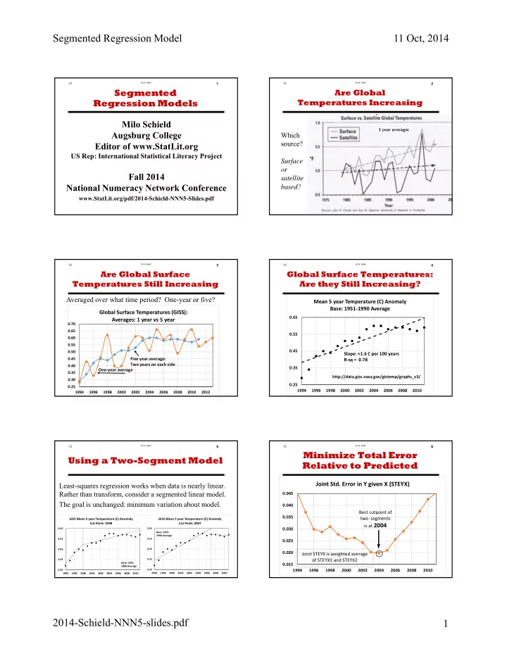
Milo Schield Augsburg College Editor of www.StatLit.org US Rep: International Statistical Literacy Project Fall 2014 National Numeracy Network Conference www.StatLit.org/pdf/2014-Schield-NNN5-Slides.pdf

  5. 1E 2014 NNN 2 Are Global Temperatures Increasing 1 year averages Which source? Surface or satellite based?

  6. 1E 2014 NNN 3 Are Global Surface Temperatures Still Increasing Averaged over what time period? One-year or five? Global Surface Temperatures (GISS): Averages: 1 year vs 5 year 0.70 0.65 0.60 0.55 0.50 0.45 Five ‐ year average: Two years on each side 0.40 One ‐ year average 0.35 0.30 0.25 1994 1996 1998 2000 2002 2004 2006 2008 2010 2012

  7. 1E 2014 NNN 4 Global Surface Temperatures: Are they Still Increasing? . Mean 5 year Temperature (C) Anomaly Base: 1951 ‐ 1990 Average 0.65 0.55 0.45 Slope: +1.6 C per 100 years R ‐ sq = 0.78 0.35 http://data.giss.nasa.gov/gistemp/graphs_v3/ 0.25 1994 1996 1998 2000 2002 2004 2006 2008 2010

  8. 1E 2014 NNN 5 Using a Two-Segment Model Least-squares regression works when data is nearly linear. Rather than transform, consider a segmented linear model. The goal is unchanged: minimum variation about model. GISS Mean 5 year Temperature (C) Anomaly GISS Mean 5 year Temperature (C) Anomaly Cut Point: 1998 Cut Point: 2007 0.65 0.65 Base: 1951 ‐ 1990 Average 0.55 0.55 0.45 0.45 0.35 0.35 Base: 1951 ‐ 1990 Average 0.25 0.25 1994 1996 1998 2000 2002 2004 2006 2008 2010 1994 1996 1998 2000 2002 2004 2006 2008 2010

  9. 1E 2014 NNN 6 Minimize Total Error Relative to Predicted . Joint Std. Error in Y given X (STEYX) 0.045 0.040 Best cutpoint of 0.035 two segments is at 2004 0.030 0.025 0.020 Joint STEYX is weighted average of STEYX1 and STEYX2 0.015 1994 1996 1998 2000 2002 2004 2006 2008 2010

  10. 1E 2014 NNN 7 Best fit Two-Segment Model . Two ‐ Segment Linear Model 0.70 0.65 0.60 0.55 Slope: ‐ 0.3 C 0.50 per 100 years 0.45 Best cutpoint of the 0.40 Slope: +2.8 C two segments 0.35 is at 2004 per 100 years 0.30 1995 1997 1999 2001 2003 2005 2007 2009 2011

  11. 1E 2014 NNN 8 Two-Segment Model: 95% Confidence Intervals . Segmented Modelling 95% Confidence Intervals 0.70 0.65 0.60 0.55 0.50 0.45 Cutpoint of 0.40 two segments 0.35 at 2004 0.30 1995 1997 1999 2001 2003 2005 2007 2009 2011

  12. 1E 2014 NNN 9 Is the Segmentation Statistically Significant? . Non ‐ Overlapping Confidence Intervals: Statistical Significance 0.64 0.62 0.60 0.58 New segment 0.56 is statistically Cutpoint of 0.54 significant two segments as of 2008 at 2004 0.52 2001 2002 2003 2004 2005 2006 2007 2008 2009

  13. 1E 2014 NNN 10 Conclusion Five-year averages of global surface temperatures: From 1994-2004, they trended up: 2.8 o C per century. Since 2004, they trended down: -0.3 o C per century After 2008 a statistician could say: “In 2004 - 2013, the trend in five-year averaged global surface temperatures changed from positive (2.8 C per 100 years) to negative (-0.3 C per 100 years) and this change in trend was statistically-significant.”

  14. 1E 2014 NNN 11 DATA LINE1 LINE1 Create Line1 Year Ave5yr b1 STEYX1 1994 0.29 1995 0.34 0.050 1996 0.42 0.065 0.012 1. Current row = 1995. 1997 0.45 0.056 0.014 1998 0.44 0.041 0.030 2. Fit 5 year data from 1999 0.48 0.037 0.028 1994 to current row. 2000 0.51 0.034 0.026 2001 0.51 0.030 0.028 3. Calculate slope b1 using 2002 0.53 0.028 0.028 Excel SLOPE. 2003 0.58 0.028 0.026 3. Calculate Std. Error of Y 2004 0.60 0.028 0.025 given X using Excel 2005 0.60 0.026 0.025 STEYX. 2006 0.58 0.024 0.030 2007 0.59 0.022 0.033 4. Increase current row; 2008 0.59 0.020 0.036 Repeat 2, 3 & 4. 2009 0.58 0.019 0.040 2010 0.57 0.017 0.044 Out-of-control??? 2011 0.59 0.015 0.045

Download Presentation
Download Policy: The content available on the website is offered to you 'AS IS' for your personal information and use only. It cannot be commercialized, licensed, or distributed on other websites without prior consent from the author. To download a presentation, simply click this link. If you encounter any difficulties during the download process, it's possible that the publisher has removed the file from their server.

Recommend


More recommend