[PPT] - Search-Based Agents Computing Driving Directions Appropriate in PowerPoint Presentation

SLIDE 1

1

Search-Based Agents

Appropriate in Static Environments where a

model of the agent is known and the environment allows

– prediction of the effects of actions – evaluation of goals or utilities of predicted states

Environment can be partially-observable,

stochastic, sequential, continuous, and even multi-agent, but it must be static!

We will first study the deterministic, discrete,

single-agent case.

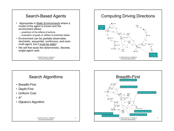
Computing Driving Directions

Arad Oradea Zerind Timisoara Lugoj Dobreta Sibiu Rimnicu Vilcea Fagaras Pitesti Mehadia Craiova Bucharest Giurgia Urzicenl Neamt Iasi Vasini Hirsova Eforie 71 75 118 140 151 99 80 111 70 75 120 146 97 138 101 211 85 90 142 92 87 98 86

You are here You want to be here

Search Algorithms

Breadth-First
Depth-First
Uniform Cost
A*
Dijkstra’s Algorithm

Oradea (146) 71

Breadth-First

Arad (0) 75 Zerind (75) 118 Timisoara (118) Lugoj (229) 111 Mehadia (299) 70 75 Dobreta (486) 120 140 Sibiu (140) 151 Rimnicu Vilcea (220) 80 Fagaras (239) 99 Craiova (366) 146 Pitesti (317) 97 138 Bucharest (450) 211 101

Detect duplicate path (291) Detect new shorter path (418) Detect duplicate path (455) Detect duplicate path (504) Detect new shorter path (374) Detect duplicate path (494) Detect duplicate path (197)

SLIDE 2

2

Breadth-First

Oradea (146) 71 Arad (0) 75 Zerind (75) 118 Timisoara (118) Lugoj (229) 111 Mehadia (299) 70 75 Dobreta (486) 120 140 Sibiu (140) 151 Rimnicu Vilcea (220) 80 Fagaras (239) 99 Craiova (366) 146 Pitesti (317) 97 138 Bucharest (450) 211 101

Arad (0) Sibiu (140) Zerind (75) Timisoara (118) Arad (150) Oradea (146) Arad (280) Fagaras (239) Oradea (291) Arad (236) Lugoj (229) Sibiu (197) Sibiu (338) Bucharest (450) Rimnicu Vilcea (220) Timisoara (340) Mehadia (299) Sibiu (300) Pitesti (317) Craiova (366) Lugoj (369) Dobreta (374) Craiova (455) Rimnicu Vilcea (317) Bucharest (418) Rimnicu Vilcea (482) Dobreta (486) Pitesti (504) Medhadia (449) Craiova (494) Zerind (217)

Formal Statement of Search Problems

State Space: set of possible “mental” states

– cities in Romania

Initial State: state from which search begins

– Arad

Operators: simulated actions that take the agent

from one mental state to another

– traverse highway between two cities

Goal Test:

– Is current state Bucharest?

General Search Algorithm

function GENERAL-SEARCH( problem, strategy) returns a solution, or failure initialize the search tree using the initial state of problem loop do if there are no candidates for expansion then return failure choose a leaf node for expansion according to strategy if the node contains a goal state then return the corresponding solution else expand the node and add the resulting nodes to the search tree end

Strategy: first-in first-out queue (expand oldest leaf first)

Leaf Selection Strategies

Breadth-First Search: oldest leaf (FIFO)
Depth-First Search: youngest leaf (LIFO)
Uniform Cost Search: cheapest leaf (Priority

Queue)

A* search: leaf with estimated shortest total path

length g(x) + h(x) = f(x)

– where g(x) is length so far – and h(x) is estimate of remaining length – (Priority Queue)

SLIDE 3

3

A* Search

Let h(x) be a “heuristic function” that gives

an underestimate of the true distance between x and the goal state

– Example: Euclidean distance

Let g(x) be the distance from the start to x,

then g(x) + h(x) is an lower bound on the length of the optimal path

Euclidean Distance Table

374 Zerind 244 Lugoj 199 Vaslui 226 Iasi 80 Urziceni 151 Hirsova 329 Timisoara 77 Giurgiu 253 Sibiu 176 Fagaras 193 Rimnicu Vilcea 161 Eforie 100 Pitesti 242 Dobreta 380 Oradea 160 Craiova 234 Neamt Bucharest 241 Mehadia 366 Arad

A* Search

Arad (0+366=366) Sibiu (140+253=393) Zerind (75+374=449) Timisoara (118+329=447) Fagaras (239+176=415) Oradea (291+380=671) Bucharest (450+0=450) Rimnicu Vilcea (220+193=413) Pitesti (317+100=417) Craiova (366+160=526) Craiova (455+160=615) Bucharest (418+0=418)

All remaining leaves have f(x) ≥ 418, so we know they cannot have shorter paths to Bucharest

Dijkstra’s Algorithm

Works backwards from the goal
Each node keeps track of the shortest

known path (and its length) to the goal

Equivalent to uniform cost search starting

at the goal

No early stopping: finds shortest path from

all nodes to the goal

SLIDE 4

4

Local Search Algorithms

Keep a single current state x
Repeat

– Apply one or more operators to x – Evaluate the resulting states according to an Objective Function J(x) – Choose one of them to replace x (or decide not to replace x at all)

Until time limit or stopping criterion

Hill Climbing

current state

bjective function

state space global maximum local maximum “flat” local maximum shoulder

Simple hill climbing:

apply a randomly-chosen

perator to the current

state

If resulting state is better,

replace current state

Steepest-Ascent Hill

Climbing:

Apply all operators to

current state, keep state with the best value

Stop when no

successors state is better than current state

Gradient Ascent

In continuous state spaces, x = (x1, x2, …, xn)

is a vector of real values

Continuous operator: x := x+ ∆x for any

arbitrary vector ∆x (infinitely many operators!)

Suppose J(x) is differentiable. Then we can

compute the direction of steepest increase of J by the first derivative with respect to x, the gradient:

Gradient Descent Search

Repeat

– Compute Gradient ∇J – Update x := x + η ∇J

Until ∇J ≈ 0
η is the “step size”, and it must be chosen

carefully

Methods such as conjugate gradient and

Newton’s method choose η automatically

SLIDE 5

5

Visualizing Gradient Ascent

If η is too large, search may overshoot and miss the maximum or

scillate forever

Problems with Hill Climbing

current state

bjective function

state space global maximum local maximum “flat” local maximum shoulder

Local optima
Flat regions
Random restarts can

give good results

Simulated Annealing

T = 100 (or some large value)
Repeat

– Apply randomly-chosen operator to x to obtain x′. – Let ∆E = J(x′) – J(x) – If ∆E > 0, switch to x′ – Else switch to x′ with probability

exp [∆E/T] (large negative steps are less likely)
T := 0.99 * T (“cool” T)
Slowly decrease T (“anneal”) to zero
Stop when no changes have been accepted for many

moves

Idea: Accept “down hill” steps with some probability to

1

Search-Based Agents

model of the agent is known and the environment allows

– prediction of the effects of actions – evaluation of goals or utilities of predicted states

stochastic, sequential, continuous, and even multi-agent, but it must be static!

single-agent case.

Computing Driving Directions

Search Algorithms

Breadth-First

2

Breadth-First

Formal Statement of Search Problems

– cities in Romania

– Arad

from one mental state to another

– traverse highway between two cities

– Is current state Bucharest?

General Search Algorithm

Leaf Selection Strategies

Queue)

length g(x) + h(x) = f(x)

– where g(x) is length so far – and h(x) is estimate of remaining length – (Priority Queue)

3

A* Search

an underestimate of the true distance between x and the goal state

– Example: Euclidean distance

then g(x) + h(x) is an lower bound on the length of the optimal path

Euclidean Distance Table

A* Search

Dijkstra’s Algorithm

known path (and its length) to the goal

at the goal

all nodes to the goal

4

Local Search Algorithms

– Apply one or more operators to x – Evaluate the resulting states according to an Objective Function J(x) – Choose one of them to replace x (or decide not to replace x at all)

Hill Climbing

Gradient Ascent

is a vector of real values

arbitrary vector ∆x (infinitely many operators!)

compute the direction of steepest increase of J by the first derivative with respect to x, the gradient:

Gradient Descent Search

– Compute Gradient ∇J – Update x := x + η ∇J

carefully

Newton’s method choose η automatically

5

Visualizing Gradient Ascent

Problems with Hill Climbing

Simulated Annealing

moves

help escape from local minima