
SLIDE 1
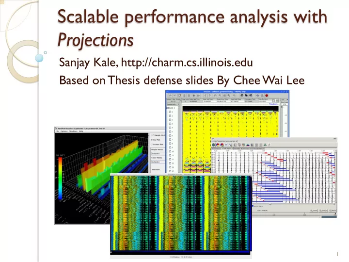
Scalable performance analysis with Projections
Sanjay Kale, http://charm.cs.illinois.edu Based on Thesis defense slides By Chee Wai Lee
1
Scalable performance analysis with Projections Sanjay Kale, - - PowerPoint PPT Presentation
Scalable performance analysis with Projections Sanjay Kale, http://charm.cs.illinois.edu Based on Thesis defense slides By Chee Wai Lee 1 Effects of Application Scaling Enlarged performance-space. Increased performance data volume.
1
2
3
4
5
6
7
8
*As we will see later, not effective with large numbers of processors.
9
10
11
12
13
14
15
16
17
18
19
20
21
Treat the vector of recorded performance metric
Measure similarity between two data points using
Given k clusters to be found, the goal is to
22
23
24
25
Metric Y Metric X Euclidean Distance Outliers Representatives
0.075 0.150 0.225 0.300 240 1200 2400 4800 9600 19200
Number of Processor Cores Seconds Time to Perform K-Means Clustering
27
28
*Chee Wai Lee, Celso Mendes and Laxmikant
Performance Analysis and Visualization through Data Reduction. 13th International Workshop on High-Level Parallel Programming Models and Supportive Environments, Miami, Florida, USA, April 2008.
29
30
31
32
33
34
512 1024 2048 4096 8192 With instrumentation, data reductions to root with remote client attached. 0.94% 0.17%
0.16% 0.83% With instrumentation, data reductions to root but no remote client attached. 0.58%
0.37% 1.14% 0.99%
35
36
37
*Isaac Dooley, Chee Wai Lee, and Laxmikant
Performance Monitoring for Large-Scale Parallel Applications. Accepted for publication at HiPC 2009, December-2009.
38
39
40
41
42
43
44
45
46
Future: a lot more emphasis on moriens (death-bed)
More “Automated Expert Analysis”
Message-driven execution or communication layer
Another grand challenge/s:
All our work has been (mostly) unfunded or only indirectly funded
47