Sampling Theory The world is continuous Like it or not, images - PDF document

Sampling Theory • The world is continuous • Like it or not, images are discrete. Intro to Sampling Theory – We work using a discrete array of pixels – We use discrete values for color – We use discrete arrays and subdivisions for specifying textures and surfaces • Process of going from continuous to discrete is called sampling. Sampling Theory Sampling Theory • Signal - function that conveys information • Point Sampling – Audio signal (1D - function of time) – start with continuous signal – Image (2D - function of space) – calculate values of signal at discrete, evenly spaced points (sampling) • Continuous vs. 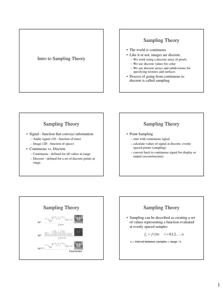Discrete – convert back to continuous signal for display or – Continuous - defined for all values in range output (reconstruction) – Discrete - defined for a set of discrete points in range. Sampling Theory Sampling Theory • Sampling can be described as creating a set of values representing a function evaluated at evenly spaced samples = ∆ = K f n f ( i ) i 0 , 1 , 2 , , n ∆ = interval between samples = range / n. Foley/VanDam 1

Sampling Theory Issues: • Sampling Rate = number of samples per unit • Important features of a scene may be missed • If view changes slightly or objects move = 1 f slightly, objects may move in and out of ∆ visibility. • To fix, sample at a higher rate, but how high • Example -- CD Audio does it need to be? – sampling rate of 44,100 samples/sec – ∆ = 1 sample every 2.26x10 -5 seconds Sampling Theory Sampling Theory • Rich mathematical foundation for sampling • Spatial vs frequency domains theory – Most well behaved functions can be described • Hope to give an “intuitive” notion of these as a sum of sin waves (possibly offset) at various frequencies mathematical concepts – Frequency specturm - a function by the contribution (and offset) at each frequency is describing the function in the frequency domain – Higher frequencies equate to greater detail Sampling Theory Sampling Theory • Nyquist Theorum – A signal can be properly reconstructed if the signal is sampled at a frequency (rate) that is greater than twice the highest frequency component of the signal. – Said another way, if you have a signal with highest frequency component of f h , you need at lease 2f h samples to represent this signal accurately. Foley/VanDam 2

Sampling Theory Sampling Theory • Aliasing • Example -- CD Audio – Failure to follow the Nyquist Theorum results in – sampling rate of 44,100 samples/sec aliasing . – ∆ = 1 sample every 2.26x10 -5 seconds – Aliasing is when high frequency components of a signal appear as low frequency due to inadequate • Using Nyquist Theorem sampling. – CDs can accurately reproduce sounds with • In CG: frequencies as high as 22,050 Hz. – Jaggies (edges) – Textures – Missed objects Sampling Theory Sampling Theory • Aliasing - example • Annoying Audio Applet – http://ptolemy.eecs.berkeley.edu/eecs20/week13/aliasin g.html Foley/VanDam(628) High frequencies masquerading as low frequencies Anti-Aliasing Fourier analysis • What to do in an aliasing situation • Given f(x) we can generate a function F(u) – Increase your sampling rate (supersampling) which indicates how much contribution – Decrease the frequency range of your signal each frequency u has on the function f. (Filtering) • F(u) is the Fourier Transform • Fourier Transform has an inverse • How do we determine the contribution of each frequency on our signal? 3

Sampling Theory Sampling Theory • The Fourier transform is defined as: • Fourier Transforms f(x) ∞ ∫ = − i π Inverse 2 ut F ( u ) f ( t ) e dt Fourier F(u) Fourier Transform Transform − ∞ f(x) Note: the Fourier Transform is defined in the complex plane Sampling Theory Sampling Theory • The Inverse Fourier transform is defined as: • How do we calculate the Fourier Transform? ∞ – Use Mathematics ∫ = i π 2 ut f ( t ) F ( u ) e du – For discrete functions, use the Fast Fourier Transform algorithm (FFT) − ∞ • Can filter the transform to remove offending high frequencies - partial solution to anti- aliasing Anti-aliasing -- Filtering Getting rid of High Frequencies • Filtering -- Frequency domain • Removes high component frequencies from – Place function into frequency domain F(u) a signal. – Simple multiplication with box filter S(u), aka pulse • Removing high frequencies results in function , band(width) limiting or low-pass filter. removing detail from the signal. − ≤ ≤ ⎧ 1 , when k u k • Can be done in the frequency or spatial = ⎨ S ( u ) ⎩ domain 0 , elsewhere – Suppress all frequency components above some specified cut-off point k 4

Filtering – Frequency Domain Getting Rid of High Frequencies Original Spectrum • Filtering -- Spatial Domain – Convolution (* operator) - equivalent to multiplying Low-Pass Filter two Fourier transforms ∞ ∫ = ∗ = τ − τ τ Spectrum with Filter h ( x ) f ( x ) g ( x ) f ( ) g ( x ) d − ∞ Taking a weighted average of the neighborhood Filtered Spectrum around each point of f , weighted by g (the convolution or filter kernel ) centered at that point. Foley/VanDam(631) Filtering using Convolution Convultion sinc Function Original Spectrum • Convolving with a sinc function in the spatial domain is the same as using a box filter in the frequency Sinc Filter domain FT → Spectrum with Filter value of filtered signal Filtered Spectrum ← FT -1 Foley/VanDam (634) Foley/VanDam (633) Convolution Sampling Theory • Joy of Convolution applet • Anti-aliasing -- Filtering – Removes high component frequencies from a signal. http://www.jhu.edu/~Esignals/convolve/index.html – Removing high frequencies results in removing detail from the signal. – Can be done in the frequency or spatial domain 5

Sampling Theory Sampling Theory • 2D Sampling • 2D Aliasing – Images are examples of sampling in 2- dimensions. – 2D Fourier Transforms provides strength of signals at frequencies in the horizontal and vertical directions aliased image anti-aliased image Foley/VanDam Sampling Theory Sampling Theory • 2D Fourier Transform ∞ ∞ � � � � ∫ ∫ − π + = i 2 ( ux vy ) F ( u , v ) f ( x , y ) e dxdy − ∞ − ∞ Castleman Sampling Theory Sampling Theory • Filtering - Convolution in 2D • Filtering – Convolution with images Castleman Castleman 6

Sampling Theory Other Anti-aliasing Methods • Filtering – Convolution in frequency domain • Pre-filtering - filtering at object precision before calculating pixel’s sample • Post-filtering - supersampling (as we’ve seen) • Adaptive supersampling - sampling rate is varied, applied only when needed (changes, edges, small items) Image 2D FFT Filter out Filtered • Stochastic supersampling - places samples at high 2D FFT stocastically determined positions rather than regular frequencies grid Castleman Anti-Aliasing Sampling Theory • Summary • Applet – Digital images are discrete with finite resolution…the http://www.nbb.cornell.edu/neurobio/land/OldStu world is not. dentProjects/cs490- – Spatial vs. Frequency domain 96to97/anson/AntiAliasingApplet/index.html – Nyquist Theorum – Convolution and Filtering – 2D Convolution & Filtering – Questions? Sampling Theory Remember • Further Reading • Class Web Site: – Foley/VanDam – Chapter 14 – http://www.cs.rit.edu/~jmg/cgII – Digital Image Processing by Kenneth • Any questions? Castleman – Glassner, Unit II (Book 1) 7