Sampling Sampling In [1]: % matplotlib inline from matplotlib - PowerPoint PPT Presentation

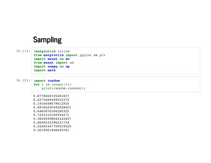
Sampling Sampling In [1]: % matplotlib inline from matplotlib import pyplot as plt import mxnet as mx from mxnet import nd import numpy as np import math In [2]: import random for i in range(10): print(random.random()) 0.8778660335481027 0.6273669409016372 0.1916048679612935 0.09766200492928401 0.6482876396284325 0.7252315169394271 0.38240498644322407 0.6658533396231734 0.25690347700919525 0.3610061946649761

Uniform Distribution Uniform Distribution In [3]: for i in range(10): print(random.randint(1, 100)) 41 39 7 9 89 75 28 40 8 49

In [4]: counts = np.zeros(100) fig, axes = plt.subplots(2, 3, figsize=(15, 8), sharex= True ) axes = axes.reshape(6) for i in range(1, 1000001): counts[random.randint(0, 99)] += 1 if i in [10, 100, 1000, 10000, 100000, 1000000]: axes[int(math.log10(i))-1].bar(np.arange(1, 101), counts) plt.show()

Categorical Distribution Categorical Distribution In [5]: # number of samples n = 1000000 y = np.random.uniform(0, 1, n) x = np.arange(1, n+1) # count number of occurrences and divide by the number of total draws p0 = np.cumsum(y < 0.35) / x p1 = np.cumsum(y >= 0.35) / x

In [6]: plt.figure(figsize=(15, 8)) plt.semilogx(x, p0) plt.semilogx(x, p1) plt.show()

Normal Distribution Normal Distribution In [7]: x = np.arange(-10, 10, 0.01) p = (1/math.sqrt(2 * math.pi)) * np.exp(-0.5 * x**2) plt.figure(figsize=(10, 5)) plt.plot(x, p) plt.show()

Central Limit Theorem in Action Central Limit Theorem in Action In [8]: # generate 10 random sequences of 10,000 uniformly distributed random variables tmp = np.random.uniform(size=(10000,10)) x = 1.0 * (tmp > 0.3) + 1.0 * (tmp > 0.8) mean = 1 * 0.5 + 2 * 0.2 variance = 1 * 0.5 + 4 * 0.2 - mean**2 print('mean {} , variance {} '.format(mean, variance)) # cumulative sum and normalization y = np.arange(1,10001).reshape(10000,1) z = np.cumsum(x,axis=0) / y mean 0.9, variance 0.49

In [9]: plt.figure(figsize=(10,5)) for i in range(10): plt.semilogx(y,z[:,i]) plt.semilogx(y,(variance**0.5) * np.power(y,-0.5) + mean,'r') plt.semilogx(y,-(variance**0.5) * np.power(y,-0.5) + mean,'r') plt.show()