Risk and Return Fundamentals In most important financial/investment - - PowerPoint PPT Presentation

8-1

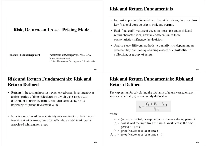
Risk, Return, and Asset Pricing Model

Nattawut Jenwittayaroje, PhD, CFA

NIDA Business School National Institute of Development Administration

Financial Risk Management

8-2

Risk and Return Fundamentals

• In most important financial/investment decisions, there are two

key financial considerations: risk and return.

• Each financial/investment decision presents certain risk and

return characteristics, and the combination of these characteristics influence the decision.

• Analysts use different methods to quantify risk depending on

whether they are looking at a single asset or a portfolio—a collection, or group, of assets.

8-3

Risk and Return Fundamentals: Risk and Return Defined

• Return is the total gain or loss experienced on an investment over

a given period of time; calculated by dividing the asset’s cash distributions during the period, plus change in value, by its beginning-of-period investment value.

• Risk is a measure of the uncertainty surrounding the return that an

investment will earn or, more formally, the variability of returns associated with a given asset.

8-4

Risk and Return Fundamentals: Risk and Return Defined

The expression for calculating the total rate of return earned on any asset over period t, rt, is commonly defined as where rt = (actual, expected, or required) rate of return during period t Ct = cash (flow) received from the asset investment in the time period t – 1 to t Pt = price (value) of asset at time t Pt – 1 = price (value) of asset at time t – 1

8-5

Risk and Return Fundamentals: Risk and Return Defined (cont.)

At the beginning of the year, Apple stock traded for $90.75 per share, and Wal-Mart was valued at $55.33. During the year, Apple paid no dividends, but Wal-Mart shareholders received dividends of $1.09 per share. At the end of the year, Apple stock was worth $210.73 and Wal-Mart sold for $52.84. We can calculate the annual rate of return, r, for each stock. Apple: ($0 + $210.73 – $90.75) ÷ $90.75 = 132.2% Wal-Mart: ($1.09 + $52.84 – $55.33) ÷ $55.33 = –2.5%

8-6

Expected Return of a Single Asset: Calculation

• Expected value of a return (r), expected return, is the average

return that an investment is expected to produce over time. where rj = return for the jth outcome Prj = probability of occurrence of the jth outcome n = number of outcomes considered

8-7

Expected Return of a Single Asset: Calculation (con’t)

Norman Company wants to choose the better of two investments, A and B. Each requires an initial outlay of $10,000. Norman Company’s past estimates indicate that the probabilities of the pessimistic, most likely, and

• ptimistic outcomes are 25%, 50%, and 25%, respectively.

(25%) (50%) (25%)

8-8

Expected Return of a Single Asset: Calculation (con’t)

8-9

Historical Returns on Selected Investments (1900–2009)

8-10

Risk of a Single Asset: Risk Assessment

• Scenario analysis is an approach for assessing risk that uses

several possible alternative outcomes (scenarios) to obtain a sense of the variability among returns.

– One common method involves considering pessimistic (worst), most likely (expected), and optimistic (best) outcomes and the returns associated with them for a given asset.

• Range is a measure of an asset’s risk, which is found by

subtracting the return associated with the pessimistic (worst)

• utcome from the return associated with the optimistic (best)
• utcome.

8-11

Risk of a Single Asset: Risk Assessment (cont.)

A bar chart is the simplest type of probability distribution; shows

• nly a limited number of outcomes and associated probabilities for a

given event. From the Norman Company example, bar charts for asset A’s and asset B’s returns are as follows;

8-12

Risk of a Single Asset: Risk Assessment (cont.)

So, Asset D is more risky than Asset C. A continuous probability distribution is a probability distribution showing all the possible outcomes and associated probabilities for a given event.

8-13

Risk of a Single Asset: Standard Deviation

Standard deviation (r) is the most common statistical indicator of an asset’s risk; it measures the dispersion around the expected value. The expression for the standard deviation of returns, r, is In general, the higher the standard deviation, the greater the risk.

8-14

The Calculation of the Standard Deviation of the Returns for Assets A and B

8-15

Historical Returns and Standard Deviations on Selected Investments (1900–2009)

• Investments with higher returns have higher standard deviations. For

example, stocks have the highest average return, but also are much more volatile.

• The historical data confirm the existence of a positive relationship

between risk and return.

8-16

Bell-Shaped Curve

• Normal probability distribution  a symmetrical probability

distribution whose shape resembles a bell-shaped curve.

8-17

Risk of a Single Asset: Standard Deviation (cont.)

Using the data in Table 8.5 and assuming that the probability distributions of returns for common stocks and bonds are normal, we can assume that:

– 68% of the possible outcomes would have a return ranging between – 11.1% and 29.7% for stocks and between –5.2% and 15.2% for bonds – 95% of the possible return outcomes would range between –31.5% and 50.1% for stocks and between –15.4% and 25.4% for bonds – The greater risk of stocks is clearly reflected in their much wider range of possible returns for each level of confidence (68% or 95%).

8-18

Risk and Return Fundamentals: Risk Preferences

Economists use three categories to describe how investors respond to risk.

– Risk averse is the attitude toward risk in which investors would require an increased return as compensation for an increase in risk  describes the behavior of most people most of the time. – Risk-neutral is the attitude toward risk in which investors choose the investment with the higher return regardless of its risk. – Risk-seeking is the attitude toward risk in which investors prefer investments with greater risk even if they have lower expected returns.

8-19

Return of a Portfolio

The return on a portfolio is a weighted average of the returns on the individual assets from which it is formed. where wj = proportion of the portfolio’s total dollar value represented by asset j rj = return on asset j

8-20

Return of a Portfolio (Con’t)

James purchases 100 shares of Wal-Mart at a price of $55 per share, so his total investment in Wal-Mart is $5,500. He also buys 100 shares of Cisco Systems at $25 per share, so the total investment in Cisco stock is $2,500.

– Combining these two holdings, James’ total portfolio is worth $8,000. – Of the total, 68.75% is invested in Wal-Mart ($5,500/$8,000) and 31.25% is invested in Cisco Systems ($2,500/$8,000). – Thus, w1 = 0.6875, w2 = 0.3125, and w1 + w2 = 1.0.

8-21

Risk of a Portfolio: Portfolio Return and Standard Deviation (Con’t)

Assume that we wish to determine the expected value and standard deviation of returns for portfolio XY, created by combining equal portions(50%) of assets X and Y. The forecasted returns of assets X and Y for each of the next 5 years (2013-2017) are illustrated in Table 8.6.

8-22

Risk of a Portfolio: Portfolio Return and Standard Deviation (Con’t)

In case of using historical data to estimate the standard deviation

8-23

Risk of a Portfolio: Correlation

• Correlation is a statistical measure of the relationship (i.e., moving

together) between any two series of numbers.

– Positively correlated describes two series that move in the same direction. – Negatively correlated describes two series that move in opposite directions.

• The correlation coefficient is a measure of the degree of

correlation between two series.

– Perfectly positively correlated describes two positively correlated series that have a correlation coefficient of +1. See Figure 8.4. – Perfectly negatively correlated describes two negatively correlated series that have a correlation coefficient of –1. See Figure 8.4.

8-24

Risk of a Portfolio: Correlation

8-25

Risk of a Portfolio: Diversification

• To reduce overall risk, it is best to diversify by combining, or adding

to the portfolio, assets that have the lowest possible correlation.

• Combining assets that have a low correlation with each other can

reduce the overall variability of a portfolio’s returns.

• Both F and G have the same average return. However, when F’s return

is above average, the return on G is below average, and vice versa.

• When these two assets are combined in a portfolio, the risk of that

portfolio falls without reducing the average return of the portfolio.

8-26

Risk of a Portfolio: Diversification

• For risk averse investors, this is very good news. They get rid
• f risk without having to sacrifice return.
• Even if assets are positively correlated, the lower the

correlation between them, the greater the risk reduction that can be achieved through diversification.

8-27

Forecasted Returns, Expected Values, and Standard Deviations for Assets X, Y, and Z and Portfolios XY and XZ

8-28

Risk of a Portfolio: Correlation, Diversification, Risk, and Return Consider two assets—Lo and Hi—with the characteristics described in the table below:

8-29

Figure 8.6: Possible Correlations

8-30

Risk of a Portfolio: International Diversification

• One excellent practical example of portfolio diversification

involves including assets from countries with business cycles that are not highly correlated with the U.S. business cycle reduces the portfolio’s responsiveness to market movements.

• Over long periods, internationally diversified portfolios tend to

perform better (meaning that they earn higher returns relative to the risks taken) than purely domestic portfolios.

8-31

Global Focus

An International Flavor to Risk Reduction

– Elroy Dimson, Paul Marsh, and Mike Staunton calculated the historical returns on a portfolio that included U.S. stocks as well as stocks from 18 other countries. – This diversified portfolio produced returns that were not quite as high as the U.S. average (9.3%), just 8.6% per year. – However, the globally diversified portfolio was also less volatile, with an annual standard deviation of 17.8% (compared with 20.4% invested in US only) – Dividing the standard deviation by the annual return produces a coefficient of variation for the globally diversified portfolio

• f 2.07, slightly lower than the 2.10 coefficient of variation

reported for U.S. stocks in Table 8.5.

8-32

Risk and Return: The Capital Asset Pricing Model (CAPM)

• The capital asset pricing model (CAPM) is the basic theory

that links risk and return for all assets.

• The CAPM quantifies the relationship between risk and

return.

• In other words, it measures how much additional return an

investor should expect from taking a little extra risk.

8-33

Risk and Return: The CAPM: Types of Risk

• Total risk is the combination of a security’s nondiversifiable risk and

diversifiable risk. – Total security risk = Diversifiable risk + Nondiversifiable risk

• Diversifiable risk is the portion of an asset’s risk that is attributable

to firm-specific, random causes; can be eliminated through

• diversification. Also called unsystematic risk.
• Nondiversifiable risk is the relevant portion of an asset’s risk

attributable to market factors that affect all firms; cannot be eliminated through diversification. Also called systematic risk.

• Because any investor can create a portfolio of assets that will

eliminate virtually all diversifiable risk, the only relevant risk is nondiversifiable risk.

8-34

Figure 8.7 Risk Reduction

8-35

Risk and Return: The CAPM: Types of Risk Unsystematic Risks Systematic Risks

8-36

Risk and Return: The CAPM

• The capital asset pricing model (CAPM) links nondiversifiable

risk and return for all assets.

• The beta coefficient (b) is a relative measure of nondiversifiable
• risk. An index of the degree of movement of an asset’s return in

response to a change in the market return.

– An asset’s historical returns are used in finding the asset’s beta

• coefficient.  Figure 8.8.

– The beta coefficient for the entire market equals 1.0. All other betas are viewed in relation to this value.

• The market return is the return on the market portfolio of all

traded securities, e.g., S&P500, SET index.

Risk and Return: The CAPM Beta estimation

37

วัน ราคาหุ้น S ราคา SET Index

20 มีค 57 300 1,355 19 มีค 57 294 1,340 18 มีค 57 296 1,350 17 มีค 57 290 1,330 14 มีค 57 288 1,325 13 มีค 57 289 1,328 . . . . . . . . .

rs

(300-294)/294 = 2.04% (294-296)/296 = -0.68% 2.07% 0.69%

• 0.35%

. . . .

rm

(1,355-1,340)/1,340 = 1.12% (1,340-1,350)/1,350 = -0.74% 1.50% 0.38%

• 0.23%

. . . .

การประมาณค่า b จากสมการ regression

ผลตอบแทนของหุ้นสามัญบริษัท s, rs

ผลตอบแทนของหุ้นสามัญโดยรวม, rm

rs = a + bsRm + e

Slope = bs

38

Risk and Return: The CAPM

8-39

Table 8.8: Selected Beta Coefficients and Their Interpretations

8-40

Table 8.9: Beta Coefficients for Selected Stocks (June 7, 2010)

8-41

Risk and Return: The CAPM (cont.)

• The beta of a portfolio can be estimated by using the betas
• f the individual assets it includes.
• Letting wj represent the proportion of the portfolio’s total

dollar value represented by asset j, and letting bj equal the beta of asset j, we can use the following equation to find the portfolio beta, bp:

8-42

Table 8.10: Mario Austino’s Portfolios V and W

The betas for the two portfolios, bv and bw, can be calculated as follows:

bv = (0.10  1.65) + (0.30  1.00) + (0.20  1.30) + (0.20  1.10) + (0.20  1.25) = 0.165 + 0.300 +0 .260 + 0.220 + 0.250 = 1.195 ≈ 1.20 bw = (0.10  .80) + (0.10  1.00) + (0.20  .65) + (0.10  .75) + (0.50  1.05) = 0.080 + 0.100 + 0.130 +0 .075 + 0.525 = 0.91

8-43

Risk and Return: The CAPM (cont.)

Using the beta coefficient to measure nondiversifiable risk, the capital asset pricing model (CAPM) is given in the following equation:

rj = RF + [bj  (rm – RF)]

where

rt = required return on asset j RF = risk-free rate of return, commonly measured by the return

• n a U.S. Treasury bill

bj = beta coefficient or index of nondiversifiable risk for asset j rm = market return; return on the market portfolio of assets (e.g., S&P500 index, SET index)

8-44

Risk and Return: The CAPM (cont.)

The CAPM can be divided into two parts:

• 1. The risk-free rate of return, (RF) which is the required

return on a risk-free asset, typically a 3-month U.S. Treasury bill.

• 2. The risk premium.
• The (rm – RF) portion of the risk premium is called the

market risk premium, because it represents the premium the investor must receive for taking the average amount of risk associated with holding the market portfolio of assets.

8-45

Risk and Return: The CAPM (cont.)

Historical Risk Premium

From the above historical data, Rf is estimated to be 3.9%, and market risk premium is 5.4%

8-46

Risk and Return: The CAPM (cont.)

Benjamin Corporation, a growing computer software developer, wishes to determine the required return on asset Z, which has a beta

• f 1.5. The risk-free rate of return is 7%; the return on the market

portfolio of assets is 11%. Substituting bZ = 1.5, RF = 7%, and rm = 11% into the CAPM yields a return of: rZ = 7% + [1.5  (11% – 7%)] = 7% + 6% = 13%