recap: Approximation Versus Generalization VC Analysis - PowerPoint PPT Presentation

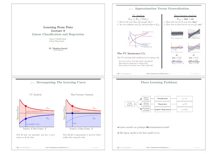
recap: Approximation Versus Generalization VC Analysis Bias-Variance Analysis E out ≤ E in + Ω( d vc ) E out = bias + var 1. Did you fit your data well enough ( E in )? 1. How well can you fit your data ( bias )? 2. Are you confident your E in will generalize to E out 2. How close to that best fit can you get ( var )? Learning From Data Lecture 8 out-of-sample error Linear Classification and Regression y y model complexity Error Linear Classification x x Linear Regression in-sample error d ∗ VC dimension, d vc g ( x ) ¯ vc y y M. Magdon-Ismail ¯ g ( x ) sin( x ) sin( x ) CSCI 4100/6100 x x The VC Insuarance Co. H 0 H 1 The VC warranty had conditions for becoming void: bias = 0 . 50; bias = 0 . 21; var = 0 . 25. var = 1 . 69. You can’t look at your data before choosing H . E out = 0 . 75 � E out = 1 . 90 Data must be generated i.i.d from P ( x ). Data and test case from same P ( x ) (same bin). � A M Linear Classification and Regression : 2 /23 c L Creator: Malik Magdon-Ismail Recap: learning curve − → recap: Decomposing The Learning Curve Three Learning Problems VC Analysis Bias-Variance Analysis Approve y = ± 1 Classification or Deny Credit Amount Regression y ∈ R Analysis of Credit Expected Error Expected Error E out E out Probability Logistic Regression y ∈ [0 , 1] of Default variance generalization error E in E in bias in-sample error • Linear models are perhaps the fundamental model. Number of Data Points, N Number of Data Points, N • The linear model is the first model to try. Pick H that can generalize and has a good Pick ( H , A ) to approximate f and not behave chance to fit the data wildly after seeing the data � A c M Linear Classification and Regression : 3 /23 � A c M Linear Classification and Regression : 4 /23 L Creator: Malik Magdon-Ismail 3 learning problems − → L Creator: Malik Magdon-Ismail Linear signal − →

The Linear Signal The Linear Signal   → sign( w t x ) linear in x : gives the line/hyperplane separator  {− 1 , +1 }      ↓         → w t x s = w t x − → s = w t x R       ↑      → θ ( w t x )  [0 , 1]   linear in w : makes the algorithms work  x is the augmented vector: x ∈ { 1 } × R d y = θ ( s ) � A M Linear Classification and Regression : 5 /23 � A M Linear Classification and Regression : 6 /23 c L Creator: Malik Magdon-Ismail Using the linear signal − → c L Creator: Malik Magdon-Ismail Classification and PLA − → Linear Classification Non-Separable Data � h ( x ) = sign( w t x ) � H lin = 1. E in ≈ E out because d vc = d + 1, �� � d E out ( h ) ≤ E in ( h ) + O N log N . 2. If the data is linearly separable, PLA will find a separator = ⇒ E in = 0. w ( t + 1) = w ( t ) + x ∗ y ∗ ↑ misclassified data point E in = 0 = ⇒ E out ≈ 0 ( f is well approximated by a linear fit). What if the data is not separable ( E in = 0 is not possible)? pocket algorithm How to ensure E in ≈ 0 is possible? select good features � A c M Linear Classification and Regression : 7 /23 � A c M Linear Classification and Regression : 8 /23 L Creator: Malik Magdon-Ismail Non-separable data − → L Creator: Malik Magdon-Ismail Pocket algorithm − →

The Pocket Algorithm Digits Data Minimizing E in is a hard combinatorial problem. The Pocket Algorithm – Run PLA – At each step keep the best E in (and w ) so far. (Its not rocket science, but it works.) Each digit is a 16 × 16 image. (Other approaches: linear regression, logistic regression, linear programming . . . ) � A M Linear Classification and Regression : 9 /23 � A M Linear Classification and Regression : 10 /23 c L Creator: Malik Magdon-Ismail Digits − → c L Creator: Malik Magdon-Ismail Input is 256 dimensional − → Digits Data Intensity and Symmetry Features feature : an important property of the input that you think is useful for classification. ( dictionary.com : a prominent or conspicuous part or characteristic) Each digit is a 16 × 16 image. � -1 -1 -1 -1 -1 -1 -1 -0.63 0.86 -0.17 -1 -1 -1 -1 -1 -1 -1 -1 -1 -1 -1 -1 -0.99 0.3 1 0.31 -1 -1 -1 -1 -1 -1 -1 -1 -1 -1 -1 -1 -0.41 1 0.99 -0.57 -1 -1 -1 -1 -1 -1 -1 -1 -1 -1 -1 -0.68 0.83 1 0.56 -1 -1 -1 -1 -1 -1 -1 -1 -1 -1 -1 -0.94 0.54 1 0.78 -0.72 -1 -1 -1 -1 -1 -1 -1 -1 -1 -1 -1 0.1 1 0.92 -0.44 -1 -1 -1 -1 -1 -1 -1 -1 -1 -1 -1 -0.26 0.95 1 -0.16 -1 -1 -1 -0.99 -0.71 -0.83 -1 -1 -1 -1 -1 -0.8 0.91 1 0.3 -0.96 -1 -1 -0.55 0.49 1 0.88 0.09 -1 -1 -1 -1 0.28 1 0.88 -0.8 -1 -0.9 0.14 0.97 1 1 1 0.99 -0.74 -1 -1 -0.95 0.84 1 0.32 -1 -1 0.35 1 0.65 -0.10 -0.18 1 0.98 -0.72 -1 -1 -0.63 1 1 0.07 -0.92 0.11 0.96 0.30 -0.88 -1 -0.07 1 0.64 -0.99 -1 -1 -0.67 1 1 0.75 0.34 1 0.70 -0.94 -1 -1 0.54 1 0.02 -1 -1 -1 -0.90 0.79 1 1 1 1 0.53 0.18 0.81 0.83 0.97 0.86 -0.63 -1 -1 -1 -1 -0.45 0.82 1 1 1 1 1 1 1 1 0.13 -1 -1 -1 -1 -1 � -1 -0.48 0.81 1 1 1 1 1 1 0.21 -0.94 -1 -1 -1 -1 -1 -1 -1 -0.97 -0.42 0.30 0.82 1 0.48 -0.47 -0.99 -1 -1 -1 -1 � x = (1 , x 1 , x 2 ) ← input � x = (1 , x 1 , · · · , x 256 ) ← input d vc = 3 d vc = 257 w = ( w 0 , w 1 , w 2 ) ← linear model w = ( w 0 , w 1 , · · · , w 256 ) ← linear model � A c M Linear Classification and Regression : 11 /23 � A c M Linear Classification and Regression : 12 /23 L Creator: Malik Magdon-Ismail Intensity and symmetry features − → L Creator: Malik Magdon-Ismail PLA on digits data − →

PLA on Digits Data Pocket on Digits Data PLA PLA Pocket 50% 50% 50% E out E out Error (log scale) Error (log scale) Error (log scale) 10% 10% 10% E out 1% 1% 1% E in E in E in 0 0 0 250 500 750 1000 250 500 750 1000 250 500 750 1000 Iteration Number, t Iteration Number, t Iteration Number, t � A M Linear Classification and Regression : 13 /23 � A M Linear Classification and Regression : 14 /23 c L Creator: Malik Magdon-Ismail Pocket on digits data − → c L Creator: Malik Magdon-Ismail Regression − → Linear Regression Linear Regression age 32 years age 32 years gender male gender male salary 40,000 salary 40,000 debt 26,000 debt 26,000 years in job 1 year years in job 1 year years at home 3 years years at home 3 years . . . . . . . . . . . . Classification: Approve/Deny Classification: Approve/Deny Regression: Credit Line (dollar amount) regression ≡ y ∈ R Regression: Credit Line (dollar amount) regression ≡ y ∈ R d d � � w i x i = w t x h ( x ) = h ( x ) = w i x i = w t x i =0 i =0 � A c M Linear Classification and Regression : 15 /23 � A c M Linear Classification and Regression : 16 /23 L Creator: Malik Magdon-Ismail Regression − → L Creator: Malik Magdon-Ismail Squared error − →

Least Squares Linear Regression Least Squares Linear Regression y y y y x 1 x 1 x 2 x 2 x x y = f ( x ) + ǫ ← − noisy target P ( y | x )  N �  E in ( h ) = 1 ( h ( x n ) − y n ) 2 in-sample error    N n =1 h ( x ) = w t x    E out ( h ) = E x [( h ( x ) − y ) 2 ] out-of-sample error  � A M Linear Classification and Regression : 17 /23 � A M Linear Classification and Regression : 18 /23 c L Creator: Malik Magdon-Ismail Squared error − → c L Creator: Malik Magdon-Ismail Matrix representation − → Using Matrices for Linear Regression Linear Regression Solution E in ( w ) = 1         — x 1 — y 1 ˆ y 1 w t x 1 N ( w t X t X w − 2 w t X t y + y t y ) — x 2 — y 2 ˆ y 2 w t x 2         X = y = y = ˆ  =  = X w  .   .   .   .  . . . . . . . .       — x N — y N y N ˆ w t x N Vector Calculus: To minimize E in ( w ), set ∇ w E in ( w ) = 0 . ∇ w ( w t A w ) = (A + A t ) w , ∇ w ( w t b ) = b . A = X t X and b = X t y : � �� � � �� � � �� � target vector in-sample predictions data matrix, N × ( d + 1) ∇ w E in ( w ) = 2 N N (X t X w − X t y ) E in ( w ) = 1 � y n − y n ) 2 (ˆ N n =1 | 2 1 = N | | ˆ y − y | Setting ∇ E in ( w ) = 0 : 2 X t X w = X t y ← − normal equations 1 | 2 = N | | X w − y | 2 1 = N ( w t X t X w − 2 w t X t y + y t y ) w lin = (X t X) − 1 X t y ← − when X t X is invertible � A c M Linear Classification and Regression : 19 /23 � A c M Linear Classification and Regression : 20 /23 L Creator: Malik Magdon-Ismail Pseudoinverse solution − → L Creator: Malik Magdon-Ismail Regression algorithm − →