Recall: Indexing into Cube Map Compute R = 2( N V ) N V Object at - - PowerPoint PPT Presentation

1

Recall: Indexing into Cube Map

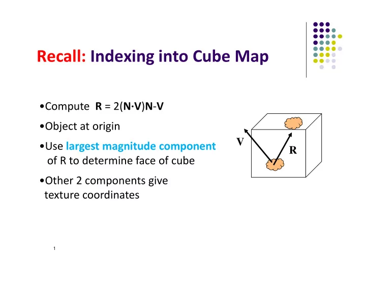
V R

• Compute R = 2(N∙V)N‐V
• Object at origin
• Use largest magnitude component
• f R to determine face of cube
• Other 2 components give

texture coordinates

Cube Map Layout

Example

 R = (‐4, 3, ‐1)  Same as R = (‐1, 0.75, ‐0.25)  Use face x = ‐1 and y = 0.75, z = ‐0.25  Not quite right since cube defined by x, y, z = ± 1

rather than [0, 1] range needed for texture coordinates

 Remap by from [‐1,1] to [0,1] range

 s = ½ + ½ y, t = ½ + ½ z

 Hence, s =0.875, t = 0.375

Sphere Environment Map

 Cube can be replaced by a sphere (sphere map)

Sphere Mapping

 Original environmental mapping technique  Proposed by Blinn and Newell  Uses lines of longitude and latitude to map

parametric variables to texture coordinates

 OpenGL supports sphere mapping  Requires a circular texture map equivalent to an

image taken with a fisheye lens

Sphere Map

Capturing a Sphere Map

Normal Mapping

 Store normals in texture  Very useful for making low‐resolution geometry look

like it’s much more detailed

Computer Graphics (CS 4731) Lecture 21: Shadows and Fog Prof Emmanuel Agu

Computer Science Dept. Worcester Polytechnic Institute (WPI)

Introduction to Shadows

 Shadows give information on relative positions of objects

Use just ambient component Use ambient + diffuse + specular components

Introduction to Shadows

 Two popular shadow rendering methods:

1.

Shadows as texture (projection)

2.

Shadow buffer

 Third method used in ray‐tracing (covered in grad

class)

Projective Shadows

 Oldest method: Used in early flight simulators  Projection of polygon is polygon called shadow polygon

Actual polygon Shadow polygon

Projective Shadows

 Works for flat surfaces illuminated by point light  For each face, project vertices V to find V’ of shadow polygon  Object shadow = union of projections of faces

Projective Shadow Algorithm

 Project light‐object edges onto plane  Algorithm:

 First, draw ground plane/scene using

specular+diffuse+ambient components

 Then, draw shadow projections (face by face) using only

ambient component

Projective Shadows for Polygon

1.

If light is at (xl, yl, zl)

2.

Vertex at (x, y, z)

3.

Would like to calculate shadow polygon vertex V projected

• nto ground at (xp, 0, zp)

(x,y,z) (xp,0,zp) Ground plane: y = 0

Projective Shadows for Polygon

 If we move original polygon so that light source is at origin  Matrix M projects a vertex V to give

its projection V’ in shadow polygon

                  1 1 1 1

yl

m

Building Shadow Projection Matrix

1.

Translate source to origin with T(‐xl, ‐yl, ‐zl)

2.

Perspective projection

3.

Translate back by T(xl, yl, zl)

                                             1 1 1 1 1 1 1 1 1 1 1 1

l l l l l l l

z y x z y x M

y

Final matrix that projects Vertex V onto V’ in shadow polygon

Code snippets?

 Set up projection matrix in OpenGL application

float light[3]; // location of light mat4 m; // shadow projection matrix initially identity M[3][1] = -1.0/light[1];

                  1 1 1 1

yl

M

Projective Shadow Code

 Set up object (e.g a square) to be drawn point4 square[4] = {vec4(-0.5, 0.5, -0.5, 1.0}

{vec4(-0.5, 0.5, -0.5, 1.0} {vec4(-0.5, 0.5, -0.5, 1.0} {vec4(-0.5, 0.5, -0.5, 1.0}

 Copy square to VBO  Pass modelview, projection matrices to vertex shader

What next?

 Next, we load model_view as usual then draw

• riginal polygon

 Then load shadow projection matrix, change color to

black, re‐render polygon

• 1. Load modelview

draw polygon as usual

• 2. Modify modelview with

Shadow projection matrix Re-render as black (or ambient)

Shadow projection Display( ) Function

void display( ) { mat4 mm; // clear the window glClear(GL_COLOR_BUFFER_BIT | GL_DEPTH_BUFFER_BIT); // render red square (original square) using modelview // matrix as usual (previously set up) glUniform4fv(color_loc, 1, red); glDrawArrays(GL_TRIANGLE_STRIP, 0, 4);

Shadow projection Display( ) Function

// modify modelview matrix to project square // and send modified model_view matrix to shader mm = model_view * Translate(light[0], light[1], light[2] *m * Translate(-light[0], -light[1], -light[2]); glUniformMatrix4fv(matrix_loc, 1, GL_TRUE, mm); //and re-render square as // black square (or using only ambient component) glUniform4fv(color_loc, 1, black); glDrawArrays(GL_TRIANGLE_STRIP, 0, 4); glutSwapBuffers( ); }

                                             1 1 1 1 1 1 1 1 1 1 1 1

l l l l l l l

z y x z y x M

y

Shadow Buffer Approach

 Uses second depth buffer called shadow buffer  Pros: not limited to plane surfaces  Cons: needs lots of memory  Depth buffer?

OpenGL Depth Buffer (Z Buffer)

 Depth: While drawing objects, depth buffer stores

distance of each polygon from viewer

 Why? If multiple polygons overlap a pixel, only

closest one polygon is drawn

eye

Z = 0.3 Z = 0.5

1.0 0.3 0.3 1.0 0.5 0.3 0.3 1.0 0.5 0.5 1.0 1.0 1.0 1.0 1.0 1.0

Depth

Setting up OpenGL Depth Buffer



Note: You did this in order to draw solid cube, meshes

1.

glutInitDisplayMode(GLUT_DEPTH | GLUT_RGB) instructs openGL to create depth buffer

2.

glEnable(GL_DEPTH_TEST) enables depth testing

3.

glClear(GL_COLOR_BUFFER_BIT | GL_DEPTH_BUFFER_BIT) Initializes depth buffer every time we draw a new picture

Shadow Buffer Theory

 Along each path from light

 Only closest object is lit  Other objects on that path in shadow

 Shadow buffer stores closest object on each path

Lit In shadow

Shadow Buffer Approach

 Rendering in two stages:

 Loading shadow buffer  Render the scene

Loading Shadow Buffer

 Initialize each element to 1.0  Position a camera at light source  Rasterize each face in scene updating closest object  Shadow buffer tracks smallest depth on each path

Shadow Buffer (Rendering Scene)

 Render scene using camera as usual  While rendering a pixel find:

 pseudo‐depth D from light source to P  Index location [i][j] in shadow buffer, to be tested  Value d[i][j] stored in shadow buffer

 If d[i][j] < D (other object on this path closer to light)

 point P is in shadow  lighting = ambient

 Otherwise, not in shadow

 Lighting = amb + diffuse + specular

D[i][j] D In shadow

Loading Shadow Buffer

 Shadow buffer calculation is independent of eye

position

 In animations, shadow buffer loaded once  If eye moves, no need for recalculation  If objects move, recalculation required

Soft Shadows

 Point light sources => simple hard shadows, unrealistic  Extended light sources => more realistic  Shadow has two parts:  Umbra (Inner part) => no light  Penumbra (outer part) => some light

Fog example

 Fog is atmospheric effect

 Better realism, helps determine distances

Fog

 Fog was part of OpenGL fixed function pipeline  Programming fixed function fog

 Parameters: Choose fog color, fog model  Enable: Turn it on

 Fixed function fog deprecated!!  Shaders can implement even better fog  Shaders implementation: fog applied in fragment

shader just before display

Rendering Fog

 Mix some color of fog: + color of surface:  If f = 0.25, output color = 25% fog + 75% surface color f

c

s

c ] 1 , [ ) 1 (     f f f

s f p

c c c

 f computed as function of distance z  3 ways: linear, exponential, exponential-squared  Linear:

start end p end

z z z z f   

start

z

End

z

P

z

Fog Shader Fragment Shader Example

float dist = abs(Position.z); Float fogFactor = (Fog.maxDist – dist)/ Fog.maxDist – Fog.minDist); fogFactor = clamp(fogFactor, 0.0, 1.0); vec3 shadeColor = ambient + diffuse + specular vec3 color = mix(Fog.color, shadeColor,fogFactor); FragColor = vec4(color, 1.0);

start end p end

z z z z f   

) 1 (

s f p

f f c c c   

Fog

 Exponential  Squared exponential  Exponential derived from Beer’s law

 Beer’s law: intensity of outgoing light diminishes

exponentially with distance

p f z

d

e f





2

) (

p f z

d

e f





Fog Optimizations

 f values for different depths ( )can be pre‐computed

and stored in a table on GPU

 Distances used in f calculations are planar  Can also use Euclidean distance from viewer or radial

distance to create radial fog

P

z

References

 Interactive Computer Graphics (6th edition), Angel

and Shreiner

 Computer Graphics using OpenGL (3rd edition), Hill

and Kelley

 Real Time Rendering by Akenine‐Moller, Haines and

Hoffman