R graph ics Can R Draw Graphs? My first peer review experience ... - - PowerPoint PPT Presentation

Can R Draw Graphs?

Paul Murrell

The University of Auckland

June 17 2006

R graphics

My first peer review experience ...

Reviewer’s comments

“An obvious reject, trivial, with no research component.” The article was accepted!

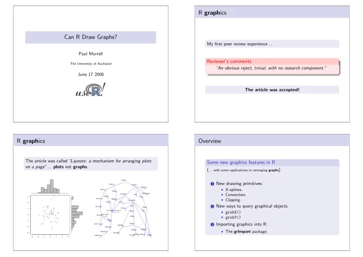
R graphics

The article was called“Layouts: a mechanism for arranging plots

• n a page”... plots not graphs.
• −3

−2 −1 1 2 3 −3 −2 −1 1 2 3

• SystemV.3

SystemV.2 SystemV.0 TS4.0 Unix.TS3.0 Unix.TS.PP CB.Unix.3 PDP11.SysV CB.Unix.2 CB.Unix.1 Unix.TS1.0 PWB2.0 USG3.0 Interdata USG2.0 PWB1.2 USG1.0 PWB1.0 FifthEd SixthEd LSX MiniUnix Wollongong SeventhEd BSD1 Xenix V32 Uniplus BSD3 BSD2 BSD4 BSD4.1 EigthEd NinethEd Ultrix32 BSD4.2 BSD4.3 BSD2.8 BSD2.9 Ultrix11 V7M

Overview

Some new graphics features in R

(... with some applications to arranging graphs)

1 New drawing primitives:

• X-splines.
• Connectors.
• Clipping.

2 New ways to query graphical objects:

• grobX()
• grobY()

3 Importing graphics into R:

• The grImport package.

X-splines

Splines are smooth curves drawn relative to a set of control

• points. Examples are Catmull-Rom splines, where the curve

interpolates the control points, and B-splines, where the curve approximates the control points. An X-spline is a smooth curve drawn relative to a set of control points, where each control point has a parameter indicating whether the curve should interpolate or approximate that particular control point. X-splines have been implemented in the grid package for R 2.3.0, via the grid.xspline() function.

grid.xspline(x, y, id, id.lengths, default.units, shape, open, arrow, repEnds, name, gp, vp)

grid.xspline()

Control points are specified as x and y locations, a shape parameter specifies interpolation or approximation at each control point, and the x-spline can be open or closed. It is also possible to add an arrow to either end of an open spline.

Open Splines

• −1

−1

• −1
• −1

1

• −1
• 1
• 1

−1

• 1
• 1

1 Closed Splines

• −1

−1 −1 −1

• −1

−1 −1

• −1

−1 1 −1

• −1
• 1
• 1

1 −1 1

• 1

1 1

• 1

1 1 1

Applications of X-Splines

• A more interesting“pointer”from a label to a feature of

interest.

• Unusual shapes.

year

Hey diddle diddle Humpty Dumpty Jack and Jill Oranges and lemons Sing a song of sixpence 1600 1650 1700 1750 1800

It's boring I'm snoring I don't like your drawing

(with apologies to "It's raining, it's pouring")

• Whether you like it or not

Your eye is drawn to this spot

(with apologies to "Hickory Dickory Dock")

Connectors

A connector is a curve drawn between two points. The function grid.curve() draws a range of connectors.

grid.curve(x1, y1, x2, y2, default.units, curvature, angle, ncp, shape, square, squareShape, inflect, arrow, debug, name, gp, vp)

Connectors

• (NULL)

(inflect = TRUE) (angle = 135) (arrow = arrow()) (ncp = 8) (shape = 0) (curvature = −1) (square = FALSE)

• (debug = TRUE)

(NULL) (inflect = TRUE) (angle = 135) (arrow = arrow()) (ncp = 8) (shape = 0) (curvature = −1) (square = FALSE)

• (debug = TRUE)

Querying Graphical Objects

It has always been possible to determine the width and height of graphical output via grobWidth() and grobHeight(). This is useful for doing things like placing decorations around text.

Hello world

It is now also possible to determine locations on the boundary of graphical output via grobX() and grobY(). grobX(x, theta) grobY(x, theta)

• Flow Diagrams

The combination of connectors and being able to determine the boundary points of objects makes it possible to create simple flow diagrams in R.

hex(.5, .8, name="h1") hex(.5, .6, name="h2") ... grid.curve(grobX("h2", 180), grobY("h2", 180), grobX("h1", 180), grobY("h1", 180), shape=1, ncp=10, square=FALSE, curvature=-1, arrow=arr) ...

A B C D

Clipping

It has always been possible to clip graphical output to a grid

• viewport. This is typically done, for example, to ensure that

plotted data do not“spill”outside the plotting region. It is now also possible to change the clipping region within a viewport, via the grid.clip() function.

x y

−1 1 2 5 10 15 20

• ●

x y

−1 1 2 5 10 15 20

• ●

x y

−1 1 2 5 10 15 20

• ●

Clipping

grid.clip(x, y, width, height, just, hjust, vjust, default.units, name, vp) ... for (i in 1:length(year)) { grid.clip(x=year[i], y=0, width=1, height=maxpop[i], "native", just="bottom") # pattern fill gridPattern() } ...

1993 1996 1998 2001 50 100 150 200 250

• Importing Graphics

R graphics can be exported in many different formats, including PDF, PostScript, PNG, and (on Windows) WMF. This is useful, for example, for including plots within larger reports. The grImport package makes it possible to go the other direction and import external graphics images for use within an R plot.

PostScript [file] PostScriptTrace() ghostscript RGML [file] readPicture() "picture" [R object] grid.picture() grid.symbols()

The PostScript Bezier Tiger

%!PS-Adobe-2.0 EPSF-1.2 %%Creator: Adobe Illustrator(TM) %%For: OpenWindows Version 2 %%Title: tiger.eps ... .8 setgray clippath fill

• 110 -300 translate

1.1 dup scale 0 g 0 G 0 i 0 J 0 j 0.172 w 10 M []0 d 0 0 0 0 k ...

Importing the Tiger

PostScriptTrace("tiger.ps") tiger <- readPicture("tiger.ps.xml")

Using the Tiger as a Plot Backdrop

pushViewport(plotViewport()) ... grid.rect() grid.xaxis(at=year) grid.yaxis() ... grid.picture(tiger) ... popViewport()

1993 1996 1998 2001 50 100 150 200 250 Estimated Population (max.) of Bengal Tigers (in Bhutan)

A Chess Board

<?xml version="1.0" encoding="UTF-8"?> <!DOCTYPE svg PUBLIC "-//W3C//DTD SVG" "http://www.w3.org/TR/2001/REC-SVG..."> <!-- Created with Sodipodi --> <svg version="1.0"> ... <g style="font-size:12;" id="g874"> <path d="M 0 437 L 437 0 " style="fill:none;fill-opacity:1" id="path616" /> ...

# Convert SVG to PostScript # using InkScape PostScriptTrace("chess.ps") chess <- readPicture("chess.ps.xml")

The Paths in the Chess Board

The picturePaths() function draws individual paths from a picture, which makes it possible to identify elements of a picture. "picture" objects can be subsetted, which makes it possible to extract elements of a picture. picturePaths(chess[125:136])

A Chess Piece as a Plotting Symbols

The number of moves required to complete chess games for different opening gambits. From the career of Louis Charles Mahe De La Bourdonnais (circa 1830).

grid.symbols( chess[205:206], x=games$num.moves, y=1:ngames, "native", size=unit(0.5, "cm"))

20 40 60 80 07 C51 Evans Gambit Match C51 Evans Gambit London m 18 C33 King's Gambit Accepted 03 D20 Queen's Gambit Accepted London B21 Sicilian, 2.f4 and 2.d4 09 C38 King's Gambit Accepted London A03 Bird's Opening 11 C51 Evans Gambit 08 C38 King's Gambit Accepted London D20 Queen's Gambit Accepted 13 C51 Evans Gambit London D20 Queen's Gambit Accepted 03 C51 Evans Gambit London C51 Evans Gambit 12 C33 King's Gambit Accepted London D20 Queen's Gambit Accepted 18 B30 Sicilian 07 C51 Evans Gambit 04 D20 Queen's Gambit Accepted London C53 Giuoco Piano 06 B21 Sicilian, 2.f4 and 2.d4 London m1 C23 Bishop's Opening

Combining Clipping and grImport

grid.picture(tiger, x=0.45, FUN=greyify) ... for (i in 1:length(year)) { grid.clip(x=year[i], y=0, width=1, height=maxpop[i], "native", just="bottom") # tiger slice grid.picture(tiger) } grid.clip() ...

1993 1996 1998 2001 50 100 150 200 250

Combining Connectors, grobX(), grobY(), and grImport

router <- readPicture("router.ps.xml") grid.picture(router, 0.5, 0.4, 0.1, 0.1, name="router2") grid.picture(router, 0.25, 0.2, 0.1, 0.1, name="router3") grid.curve(grobX("router2", 270), grobY("router2", 270), grobX("router3", 0), grobY("router3", 0))

Authentication Server Gateway Koala 9.9.9.9 15.15.15.15

Summary

grid.xspline() Draw a smooth curve relative to control points. grid.curve() Draw a connector between two end points. grid.clip() Reset the clipping region within the current viewport. grobX(), grobY() Determine a location

• n

the boundary of a graphical object. grImport Import PostScript images for draw- ing in R.

Can R draw graphs?

Depending on what you meant by“graph” , the answer used to be either“yes, of course!” or“yeeessss, sort of” . With the new features in R 2.3.0, the answer in either case is a more emphatic“yes” .

Acknowledgements

• Richard Walton made significant improvements to the grImport code last

(Southern) Summer.

• The ggm package by Giovanni Marchetti and Mathias Drton was used to

produce the example node-and-edge graph in the introduction.

• The dates of first pulication of Nursery Rhymes came from

http://www.rhymes.org.uk/ and http://www.bbc.co.uk/dna/h2g2/alabaster/A696125.

• The cartoon bubble text example was motivated by a recent R-help message by

Ivo Welch.

• The clipping example was motivated by a recent R-help message by ArrayChip.
• The tiger image is part of the ghostscript distribution; the tiger data are from

http://www.globaltiger.org/population.htm.

• The greyscale version of the tiger used the colorspace package by Ross Ihaka.
• The chess board image (by Jose Hevia) is from the Open Clip Art Library

http://openclipart.org/clipart//recreation/games/chess/chess_game_01.svg

• The chess data are from chessgames.com

http://www.chessgames.com/perl/chess.pl?page=1&pid=31596

• The network diagram used the Cisco Network Topology Icons

http://www.cisco.com/web/about/ac50/ac47/2.html