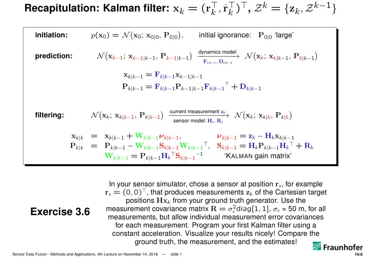
R 0 0 z 0 ( v max ) 2 1 x 0 | 0 = r 0 | 0 = P 0 | 0 = - PowerPoint PPT Presentation

k ) ⊤ , Z k = { z k , Z k − 1 } Recapitulation: Kalman filter: x k = ( r ⊤ r ⊤ k , ˙ � � p ( x 0 ) = N initiation: x 0 ; x 0 | 0 , P 0 | 0 , initial ignorance: P 0 | 0 ‘large’ N � x k − 1 ; x k − 1 | k − 1 , P k − 1 | k − 1 � dynamics model N � x k ; x k | k − 1 , P k | k − 1 � − − − − − − − − − → prediction: F k | k − 1 , D k | k − 1 x k | k − 1 = F k | k − 1 x k − 1 | k − 1 ⊤ + D k | k − 1 P k | k − 1 = F k | k − 1 P k − 1 | k − 1 F k | k − 1 � � � � current measurement z k N x k ; x k | k − 1 , P k | k − 1 − − − − − − − − − − − − − → N x k ; x k | k , P k | k filtering: sensor model: H k , R k x k | k = x k | k − 1 + W k | k − 1 ν k | k − 1 , ν k | k − 1 = z k − H k x k | k − 1 S k | k − 1 = H k P k | k − 1 H k ⊤ + R k P k | k − 1 − W k | k − 1 S k | k − 1 W k | k − 1 ⊤ , P k | k = W k | k − 1 = P k | k − 1 H k ⊤ S k | k − 1 − 1 ‘K ALMAN gain matrix’ In your sensor simulator, chose a sensor at position r s , for example r s = (0 , 0) ⊤ , that produces measurements z k of the Cartesian target positions Hx k from your ground truth generator. Use the measurement covariance matrix R = σ 2 c diag[1 , 1] , σ c = 50 m, for all Exercise 3.6 measurements, but allow individual measurement error covariances for each measurement. Program your first Kalman filter using a constant acceleration. Visualize your results nicely! Compare the ground truth, the measurement, and the estimates! Sensor Data Fusion - Methods and Applications, 4th Lecture on November 14, 2018 — slide 1

� � p ( x 0 |Z 0 ) = N x 0 ; x 0 | 0 , P 0 | 0 a first remark on initiation: , P 0 | 0 ‘large’       r 0 | 0 R 0 0 z 0   ( v max ) 2 1 ˙ x 0 | 0 = r 0 | 0  =   P 0 | 0 =   0  , 0 0       ( q max ) 2 1 0 ¨ r 0 | 0 0 0 position information: first measurement z 0 , ignorance = measurement error R ! ignorance on velocity: sphere with radius v max around zero (= no information on direction, but on ‘limits’) ignorance on acceleration: sphere with radius q max around zero Sensor Data Fusion - Methods and Applications, 4th Lecture on November 14, 2018 — slide 2

Sensor Fusion: Gain in Localization Accuracy If a stationary target is observed by N sensors, we na¨ ıvely √ expect an improvement in accuracy ∝ 1 / N . Sensor Data Fusion - Methods and Applications, 4th Lecture on November 14, 2018 — slide 3

Sensor Fusion: Gain in Localization Accuracy If a stationary target is observed by N sensors, we na¨ ıvely √ expect an improvement in accuracy ∝ 1 / N . a closer look: The error of each measurement z i is described by a related measurement error covariance matrix R i (‘error ellipsoids’). In 2 dimensions: s1 s2 s3 R i can strongly depend on the underlying senor-to-target geometry! Sensor Data Fusion - Methods and Applications, 4th Lecture on November 14, 2018 — slide 4

More Realistic: Range, Azimuth Measurements • measurements in polar coordinates: � � σ 2 r 0 z k = ( r k , ϕ k ) ⊤ , measurement error: R = , r , ϕ independent 0 σ 2 ϕ Sensor Data Fusion - Methods and Applications, 4th Lecture on November 14, 2018 — slide 5

More Realistic: Range, Azimuth Measurements • measurements in polar coordinates: � � σ 2 r 0 z k = ( r k , ϕ k ) ⊤ , measurement error: R = , r , ϕ independent 0 σ 2 ϕ Likelihood function in polar coordinates: p ( z k | x k ) = N ( z k ; x p k , R p ) Sensor Data Fusion - Methods and Applications, 4th Lecture on November 14, 2018 — slide 6

More Realistic: Range, Azimuth Measurements • measurements in polar coordinates: � � σ 2 r 0 z k = ( r k , ϕ k ) ⊤ , measurement error: R = , r , ϕ independent 0 σ 2 ϕ Likelihood function in polar coordinates: p ( z k | x k ) = N ( z k ; x p k , R p ) • What is the likelihood function in Cartesian coordinates? � cos ϕ k � t [ z k ] = r k sin ϕ k Sensor Data Fusion - Methods and Applications, 4th Lecture on November 14, 2018 — slide 7

More Realistic: Range, Azimuth Measurements • measurements in polar coordinates: � � σ 2 r 0 z k = ( r k , ϕ k ) ⊤ , measurement error: R = , r , ϕ independent 0 σ 2 ϕ • in Cartesian coord.: expand around r k | k − 1 = ( r k | k − 1 , ϕ k | k − 1 ) ⊤ : � cos ϕ k � t [ z k ] = r k ≈ t [ r k | k − 1 ] + T ( z k − r k | k − 1 ) sin ϕ k constant and linear term of a Taylor series only, blackboard! Sensor Data Fusion - Methods and Applications, 4th Lecture on November 14, 2018 — slide 8

More Realistic: Range, Azimuth Measurements • measurements in polar coordinates: � � σ 2 r 0 z k = ( r k , ϕ k ) ⊤ , measurement error: R = , r , ϕ independent 0 σ 2 ϕ • in Cartesian coord.: expand around r k | k − 1 = ( r k | k − 1 , ϕ k | k − 1 ) ⊤ : � cos ϕ k � t [ z k ] = r k ≈ t [ r k | k − 1 ] + T ( z k − r k | k − 1 ) sin ϕ k � � � � � � cos ϕ − sin ϕ 1 0 cos ϕ k | k − 1 − r k | k − 1 sin ϕ k | k − 1 T = ∂ t [ r k | k − 1 ] = = sin ϕ k | k − 1 r k | k − 1 cos ϕ k | k − 1 sin ϕ cos ϕ 0 r ∂ r k | k − 1 � �� � � �� � rotation D ϕ dilation S r Sensor Data Fusion - Methods and Applications, 4th Lecture on November 14, 2018 — slide 9

More Realistic: Range, Azimuth Measurements • measurements in polar coordinates: � � σ 2 r 0 z k = ( r k , ϕ k ) ⊤ , measurement error: R = , r , ϕ independent 0 σ 2 ϕ • in Cartesian coord.: expand around r k | k − 1 = ( r k | k − 1 , ϕ k | k − 1 ) ⊤ : � cos ϕ k � t [ z k ] = r k ≈ t [ r k | k − 1 ] + T ( z k − r k | k − 1 ) sin ϕ k � � � � � � cos ϕ − sin ϕ 1 0 cos ϕ k | k − 1 − r k | k − 1 sin ϕ k | k − 1 T = ∂ t [ r k | k − 1 ] = = sin ϕ k | k − 1 r k | k − 1 cos ϕ k | k − 1 sin ϕ cos ϕ 0 r ∂ r k | k − 1 � �� � � �� � rotation D ϕ dilation S r • affine transform of G AUSS ian random variables: N � z ; x , R � → N � z ′ ; t + Tx , TRT ⊤ � z ′ = t + Tz − − − − − − Sensor Data Fusion - Methods and Applications, 4th Lecture on November 14, 2018 — slide 10

More Realistic: Range, Azimuth Measurements • measurements in polar coordinates: � � σ 2 r 0 z k = ( r k , ϕ k ) ⊤ , measurement error: R = , r , ϕ independent 0 σ 2 ϕ • in Cartesian coord.: expand around r k | k − 1 = ( r k | k − 1 , ϕ k | k − 1 ) ⊤ : � cos ϕ k � t [ z k ] = r k ≈ t [ r k | k − 1 ] + T ( z k − r k | k − 1 ) sin ϕ k � � � � � � cos ϕ − sin ϕ 1 0 cos ϕ k | k − 1 − r k | k − 1 sin ϕ k | k − 1 T = ∂ t [ r k | k − 1 ] = = sin ϕ k | k − 1 r k | k − 1 cos ϕ k | k − 1 sin ϕ cos ϕ 0 r ∂ r k | k − 1 � �� � � �� � rotation D ϕ dilation S r • Cartesian error covariance (time dependent): � � TRT ⊤ = D ϕ S r R S r D ⊤ σ 2 0 D ⊤ ϕ = D ϕ r ϕ 0 ( rσ ϕ ) 2 • sensor fusion: sensor-to-target-geometry enters into TRT ⊤ Sensor Data Fusion - Methods and Applications, 4th Lecture on November 14, 2018 — slide 11

s1 s2 s3 sensor fusion: sensor-to-target-geometry enters into TRT ⊤ Sensor Data Fusion - Methods and Applications, 4th Lecture on November 14, 2018 — slide 12

S k Sensors Producing Target Measurement at the Same Time   H 1 k . k , . . . , R S k  .  R k = diag[ R 1 . H k x k = k ] One possibility:  x k ,    H S k k Sensor Data Fusion - Methods and Applications, 4th Lecture on November 14, 2018 — slide 13

S k Sensors Producing Target Measurement at the Same Time   H 1 k . k , . . . , R S k  .  R k = diag[ R 1 . H k x k = k ] One possibility:  x k ,    H S k k Alternatively, provided that H i k = H k , i = 1 , . . . , S k : p ( z 1 k , z 2 k | x k ) = p ( z 1 k | x k ) p ( z 2 k | x k ) independent sensors � � � � z 1 k ; H k x k , R 1 z 2 k ; H k x k , R 2 = N N k k Sensor Data Fusion - Methods and Applications, 4th Lecture on November 14, 2018 — slide 14

S k Sensors Producing Target Measurement at the Same Time   H 1 k . k , . . . , R S k  .  R k = diag[ R 1 . H k x k = k ] One possibility:  x k ,    H S k k Alternatively, provided that H i k = H k , i = 1 , . . . , S k : p ( z 1 k , z 2 k | x k ) = p ( z 1 k | x k ) p ( z 2 k | x k ) independent sensors � � � � z 1 k ; H k x k , R 1 z 2 k ; H k x k , R 2 = N N k k Sensor Data Fusion - Methods and Applications, 4th Lecture on November 14, 2018 — slide 15

A Useful Product Formula for G AUSS ians � � x ; y + W ν , P − WSW ⊤ � N � � � � � � N z ; Hx , R N x ; y , P = N z ; Hy , S × N � x ; Q − 1 ( P − 1 x + H ⊤ R − 1 z ) , Q � � �� � independent of x S = HPH ⊤ + R , Q − 1 = P − 1 + H ⊤ R − 1 H . W = PH ⊤ S − 1 , ν = z − Hy , Sensor Data Fusion - Methods and Applications, 4th Lecture on November 14, 2018 — slide 16