Quicksort Proposed by C.A.R. Hoare in 1962. Divide-and-conquer - - PowerPoint PPT Presentation

1

2/17/09 CS 5633 Analysis of Algorithms 1

CS 3343 -- Spring 2009

Quicksort

Carola Wenk Slides courtesy of Charles Leiserson with small changes by Carola Wenk

2/17/09 CS 5633 Analysis of Algorithms 2

Quicksort

• Proposed by C.A.R. Hoare in 1962.
• Divide-and-conquer algorithm.
• Sorts “in place” (like insertion sort, but not

like merge sort).

• Very practical (with tuning).

2/17/09 CS 5633 Analysis of Algorithms 3

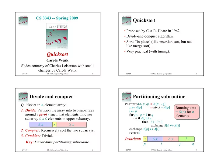
Divide and conquer

Quicksort an n-element array:

• 1. Divide: Partition the array into two subarrays

around a pivot x such that elements in lower subarray ≤ x ≤ elements in upper subarray.

• 2. Conquer: Recursively sort the two subarrays.
• 3. Combine: Trivial.

≤ x ≤ x x x ≥ x ≥ x Key: Linear-time partitioning subroutine.

2/17/09 CS 5633 Analysis of Algorithms 4

Running time = O(n) for n elements. Running time = O(n) for n elements.

Partitioning subroutine

PARTITION(A, p, q) ⊳ A[p . . q] x ← A[p] ⊳ pivot = A[p] i ← p for j ← p + 1 to q do if A[ j] ≤ x then i ← i + 1 exchange A[i] ↔ A[ j] exchange A[p] ↔ A[i] return i

x x ≤ x ≤ x ≥ x ≥ x ? ? p i q j Invariant:

2

2/17/09 CS 5633 Analysis of Algorithms 5

Example of partitioning

i j 6 6 10 10 13 13 5 5 8 8 3 3 2 2 11 11

2/17/09 CS 5633 Analysis of Algorithms 6

Example of partitioning

i j 6 6 10 10 13 13 5 5 8 8 3 3 2 2 11 11

2/17/09 CS 5633 Analysis of Algorithms 7

Example of partitioning

i j 6 6 10 10 13 13 5 5 8 8 3 3 2 2 11 11

2/17/09 CS 5633 Analysis of Algorithms 8

Example of partitioning

6 6 10 10 13 13 5 5 8 8 3 3 2 2 11 11 i j 6 6 5 5 13 13 10 10 8 8 3 3 2 2 11 11

3

2/17/09 CS 5633 Analysis of Algorithms 9

Example of partitioning

6 6 10 10 13 13 5 5 8 8 3 3 2 2 11 11 i j 6 6 5 5 13 13 10 10 8 8 3 3 2 2 11 11

2/17/09 CS 5633 Analysis of Algorithms 10

Example of partitioning

6 6 10 10 13 13 5 5 8 8 3 3 2 2 11 11 i j 6 6 5 5 13 13 10 10 8 8 3 3 2 2 11 11

2/17/09 CS 5633 Analysis of Algorithms 11

Example of partitioning

6 6 10 10 13 13 5 5 8 8 3 3 2 2 11 11 i j 6 6 5 5 3 3 10 10 8 8 13 13 2 2 11 11 6 6 5 5 13 13 10 10 8 8 3 3 2 2 11 11

2/17/09 CS 5633 Analysis of Algorithms 12

Example of partitioning

6 6 10 10 13 13 5 5 8 8 3 3 2 2 11 11 i j 6 6 5 5 3 3 10 10 8 8 13 13 2 2 11 11 6 6 5 5 13 13 10 10 8 8 3 3 2 2 11 11

4

2/17/09 CS 5633 Analysis of Algorithms 13

Example of partitioning

6 6 10 10 13 13 5 5 8 8 3 3 2 2 11 11 6 6 5 5 3 3 10 10 8 8 13 13 2 2 11 11 6 6 5 5 13 13 10 10 8 8 3 3 2 2 11 11 i j 6 6 5 5 3 3 2 2 8 8 13 13 10 10 11 11

2/17/09 CS 5633 Analysis of Algorithms 14

Example of partitioning

6 6 10 10 13 13 5 5 8 8 3 3 2 2 11 11 6 6 5 5 3 3 10 10 8 8 13 13 2 2 11 11 6 6 5 5 13 13 10 10 8 8 3 3 2 2 11 11 i j 6 6 5 5 3 3 2 2 8 8 13 13 10 10 11 11

2/17/09 CS 5633 Analysis of Algorithms 15

Example of partitioning

6 6 10 10 13 13 5 5 8 8 3 3 2 2 11 11 6 6 5 5 3 3 10 10 8 8 13 13 2 2 11 11 6 6 5 5 13 13 10 10 8 8 3 3 2 2 11 11 i j 6 6 5 5 3 3 2 2 8 8 13 13 10 10 11 11

2/17/09 CS 5633 Analysis of Algorithms 16

Example of partitioning

6 6 10 10 13 13 5 5 8 8 3 3 2 2 11 11 6 6 5 5 3 3 10 10 8 8 13 13 2 2 11 11 6 6 5 5 13 13 10 10 8 8 3 3 2 2 11 11 6 6 5 5 3 3 2 2 8 8 13 13 10 10 11 11 i 2 2 5 5 3 3 6 6 8 8 13 13 10 10 11 11

5

2/17/09 CS 5633 Analysis of Algorithms 17

Pseudocode for quicksort

QUICKSORT(A, p, r) if p < r then q ← PARTITION(A, p, r) QUICKSORT(A, p, q–1) QUICKSORT(A, q+1, r) Initial call: QUICKSORT(A, 1, n)

2/17/09 CS 5633 Analysis of Algorithms 18

Analysis of quicksort

• Assume all input elements are distinct.
• In practice, there are better partitioning

algorithms for when duplicate input elements may exist.

• Let T(n) = worst-case running time on

an array of n elements.

2/17/09 CS 5633 Analysis of Algorithms 19

Worst-case of quicksort

• Input sorted or reverse sorted.
• Partition around min or max element.
• One side of partition always has no elements.

) ( ) ( ) 1 ( ) ( ) 1 ( ) 1 ( ) ( ) 1 ( ) ( ) (

2

n n n T n n T n n T T n T Θ = Θ + − = Θ + − + Θ = Θ + − + = (arithmetic series)

2/17/09 CS 5633 Analysis of Algorithms 20

Worst-case recursion tree

T(n) = T(0) + T(n–1) + cn

6

2/17/09 CS 5633 Analysis of Algorithms 21

Worst-case recursion tree

T(n) = T(0) + T(n–1) + cn T(n)

2/17/09 CS 5633 Analysis of Algorithms 22

cn T(0) T(n–1)

Worst-case recursion tree

T(n) = T(0) + T(n–1) + cn

2/17/09 CS 5633 Analysis of Algorithms 23

cn T(0) c(n–1)

Worst-case recursion tree

T(n) = T(0) + T(n–1) + cn T(0) T(n–2)

2/17/09 CS 5633 Analysis of Algorithms 24

cn T(0) c(n–1)

Worst-case recursion tree

T(n) = T(0) + T(n–1) + cn T(0) c(n–2) T(0) Θ(1)

…

7

2/17/09 CS 5633 Analysis of Algorithms 25

cn T(0) c(n–1)

Worst-case recursion tree

T(n) = T(0) + T(n–1) + cn T(0) c(n–2) T(0) T(0)

( )

2 1

n k

k

Θ =         Θ ∑

=

height

height = n

…

2/17/09 CS 5633 Analysis of Algorithms 26

cn T(0) c(n–1)

Worst-case recursion tree

T(n) = T(0) + T(n–1) + cn T(0) c(n–2) T(0) T(0)

( )

2 1

n k

k

Θ =         Θ ∑

=

n

height = n

…

2/17/09 CS 5633 Analysis of Algorithms 27

cn c(n–1)

Worst-case recursion tree

T(n) = T(0) + T(n–1) + cn c(n–2) Θ(1)

( )

2 1

n k

k

Θ =         Θ ∑

=

n

height = n Θ(1) Θ(1) Θ(1) T(n) = Θ(n) + Θ(n2) = Θ(n2)

…

2/17/09 CS 5633 Analysis of Algorithms 28

Best-case analysis

(For intuition only!) If we’re lucky, PARTITION splits the array evenly: T(n) = 2T(n/2) + Θ(n) = Θ(n log n) (same as merge sort) What if the split is always

10 9 10 1 :

?

( ) ( )

) ( ) (

10 9 10 1

n n T n T n T Θ + + = What is the solution to this recurrence?

8

2/17/09 CS 5633 Analysis of Algorithms 29

Analysis of “almost-best” case

) (n T

2/17/09 CS 5633 Analysis of Algorithms 30

Analysis of “almost-best” case

cn

( )

n T 10

1

( )

n T 10

9

2/17/09 CS 5633 Analysis of Algorithms 31

Analysis of “almost-best” case

cn cn

10 1

cn

10 9

( )

n T 100

1

( )

n T 100

9

( )

n T 100

9

( )

n T 100

81

2/17/09 CS 5633 Analysis of Algorithms 32

Analysis of “almost-best” case

cn cn

10 1

cn

10 9

cn

100 1

cn

100 9

cn

100 9

cn

100 81

Θ(1) Θ(1) … … log10/9n cn cn cn … O(n) leaves O(n) leaves

9

2/17/09 CS 5633 Analysis of Algorithms 33

log10n

Analysis of “almost-best” case

cn cn

10 1

cn

10 9

cn

100 1

cn

100 9

cn

100 9

cn

100 81

Θ(1) Θ(1) … … log10/9n cn cn cn T(n) ≤ cnlog10/9n + Ο(n) … cnlog10n ≤ O(n) leaves O(n) leaves Θ(nlog n)

2/17/09 CS 5633 Analysis of Algorithms 34

Quicksort Runtimes

• Best case runtime Tbest(n) ∈ O(n log n)
• Worst case runtime Tworst(n) ∈ O(n2)
• Worse than mergesort? Why is it called

quicksort then?

• Its average runtime Tavg(n) ∈ O(n log n )
• Better even, the expected runtime of

randomized quicksort is O(n log n)

2/17/09 CS 5633 Analysis of Algorithms 35

Average Runtime

The average runtime Tavg(n) for Quicksort is the average runtime over all possible inputs

• f length n.
• What kind of inputs are there?
• How many inputs are there?

2/17/09 CS 5633 Analysis of Algorithms 36

Average Runtime

• What kind of inputs are there?
• Do [1,2,…,n] and [5,6,…,n+5] cause

different runtimes of Quicksort?

• No. Therefore only consider all

permutations of [1,2,…,n] .

• How many inputs are there?
• There are n! different permutations of

[1,2,…,n]

10

2/17/09 CS 5633 Analysis of Algorithms 37

Average Runtime

• Therefore, Tavg(n) has to average the runtimes
• ver all n! different input permutations
• Disadvantage of considering average runtime:
• There are still worst-case inputs that will

have a O(n2) runtime

• Are all inputs really equally likely? That

depends on the application ⇒ Better: Use randomized quicksort

2/17/09 CS 5633 Analysis of Algorithms 38

Randomized quicksort

IDEA: Partition around a random element.

• Running time is independent of the input
• rder.
• No assumptions need to be made about

the input distribution.

• No specific input elicits the worst-case

behavior.

• The worst case is determined only by the
• utput of a random-number generator.

2/17/09 CS 5633 Analysis of Algorithms 39

Randomized quicksort analysis

• T(n) = random variable for the running time of

randomized quicksort on an input of size n, assuming random numbers are independent.

• E(T(n)) = expected value of T(n), the

“expected runtime” of randomized quicksort. T(n) = T(0) + T(n–1) + Θ(n) if 0 : n–1 split, T(1) + T(n–2) + Θ(n) if 1 : n–2 split, … T(n–1) + T(0) + Θ(n) if n–1 : 0 split,

2/17/09 CS 5633 Analysis of Algorithms 40

Randomized quicksort analysis

For k = 0, 1, …, n–1, define the indicator random variable Xk = 1 if PARTITION generates a k : n–k–1 split, 0 otherwise. E[Xk] = Pr{Xk = 1} = 1/n, since all splits are equally likely, assuming elements are distinct.

11

2/17/09 CS 5633 Analysis of Algorithms 41

Analysis (continued)

T(n) = T(0) + T(n–1) + Θ(n) if 0 : n–1 split, T(1) + T(n–2) + Θ(n) if 1 : n–2 split, … T(n–1) + T(0) + Θ(n) if n–1 : 0 split,

( )

∑

− =

Θ + − − + =

1

) ( ) 1 ( ) (

n k k

n k n T k T X .

2/17/09 CS 5633 Analysis of Algorithms 42

Calculating expectation

( )

     Θ + − − + =

∑

− = 1

) ( ) 1 ( ) ( )] ( [

n k k

n k n T k T X E n T E

Take expectations of both sides.

2/17/09 CS 5633 Analysis of Algorithms 43

Calculating expectation

( ) ( ) [ ]

∑ ∑

− = − =

Θ + − − + =       Θ + − − + =

1 1

) ( ) 1 ( ) ( ) ( ) 1 ( ) ( )] ( [

n k k n k k

n k n T k T X E n k n T k T X E n T E

Linearity of expectation.

2/17/09 CS 5633 Analysis of Algorithms 44

Calculating expectation

( ) ( ) [ ] [ ] [ ]

∑ ∑ ∑

− = − = − =

Θ + − − + ⋅ = Θ + − − + =       Θ + − − + =

1 1 1

) ( ) 1 ( ) ( ) ( ) 1 ( ) ( ) ( ) 1 ( ) ( )] ( [

n k k n k k n k k

n k n T k T E X E n k n T k T X E n k n T k T X E n T E

Independence of Xk from other random choices.

12

2/17/09 CS 5633 Analysis of Algorithms 45

Calculating expectation

( ) ( ) [ ] [ ] [ ] [ ] [ ]

∑ ∑ ∑ ∑ ∑ ∑

− = − = − = − = − = − =

Θ + − − + = Θ + − − + ⋅ = Θ + − − + =       Θ + − − + =

1 1 1 1 1 1

) ( 1 ) 1 ( 1 ) ( 1 ) ( ) 1 ( ) ( ) ( ) 1 ( ) ( ) ( ) 1 ( ) ( )] ( [

n k n k n k n k k n k k n k k

n n k n T E n k T E n n k n T k T E X E n k n T k T X E n k n T k T X E n T E

Linearity of expectation; E[Xk] = 1/n.

2/17/09 CS 5633 Analysis of Algorithms 46

Calculating expectation

( ) ( ) [ ] [ ] [ ] [ ] [ ] [ ]

) ( ) ( 2 ) ( 1 ) 1 ( 1 ) ( 1 ) ( ) 1 ( ) ( ) ( ) 1 ( ) ( ) ( ) 1 ( ) ( )] ( [

1 1 1 1 1 1 1

n k T E n n n k n T E n k T E n n k n T k T E X E n k n T k T X E n k n T k T X E n T E

n k n k n k n k n k k n k k n k k

Θ + = Θ + − − + = Θ + − − + ⋅ = Θ + − − + =       Θ + − − + =

∑ ∑ ∑ ∑ ∑ ∑ ∑

− = − = − = − = − = − = − =

Summations have identical terms.

2/17/09 CS 5633 Analysis of Algorithms 47

Hairy recurrence

[ ]

) ( ) ( 2 )] ( [

1 2

n k T E n n T E

n k

Θ + = ∑

− =

(The k = 0, 1 terms can be absorbed in the Θ(n).) Prove: E[T(n)] ≤ anlogn for constant a > 0. Use fact:

2 1 2 8 1 2 2 1

log log n n n k k

n k

∑

− =

− ≤ (exercise).

• Choose a large enough so that anlogn

dominates E[T(n)] for sufficiently small n ≥ 2.

2/17/09 CS 5633 Analysis of Algorithms 48

Substitution method

[ ]

) ( log 2 ) (

1 2

n k ak n n T E

n k

Θ + ≤ ∑

− =

Substitute inductive hypothesis.

13

2/17/09 CS 5633 Analysis of Algorithms 49

Substitution method

[ ]

) ( 8 1 log 2 1 2 ) ( log 2 ) (

2 2 1 2

n n n n n a n k ak n n T E

n k

Θ +       − ≤ Θ + ≤ ∑

− =

Use fact.

2/17/09 CS 5633 Analysis of Algorithms 50

Substitution method

[ ]

      Θ − − = Θ +       − ≤ Θ + ≤ ∑

− =

) ( 4 log ) ( 8 1 log 2 1 2 ) ( log 2 ) (

2 2 1 2

n an n an n n n n n a n k ak n n T E

n k

Express as desired – residual.

2/17/09 CS 5633 Analysis of Algorithms 51

Substitution method

[ ]

n an n an n an n n n n n a n k ak n n T E

n k

log ) ( 4 log ) ( 8 1 log 2 1 2 ) ( log 2 ) (

2 2 1 2

≤       Θ − − = Θ +       − = Θ + ≤ ∑

− =

if a is chosen large enough so that an/4 dominates the Θ(n). ,

2/17/09 CS 5633 Analysis of Algorithms 52

Quicksort in practice

• Quicksort is a great general-purpose

sorting algorithm.

• Quicksort is typically over twice as fast

as merge sort.

• Quicksort can benefit substantially from

code tuning.

• Quicksort behaves well even with

caching and virtual memory.