Probabilistic Graphical Models 10-708 More on learning fully - PDF document

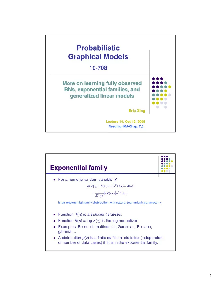
Probabilistic Graphical Models 10-708 More on learning fully observed More on learning fully observed BNs, exponential families, and , exponential families, and BNs generalized linear models generalized linear models Eric Xing Eric Xing Lecture 10, Oct 12, 2005 Reading: MJ-Chap. 7,8 Exponential family � For a numeric random variable X { } p x h x T T x A η = η − η ( | ) ( ) exp ( ) ( ) 1 { } = h x η T T x ( ) exp ( ) Z η ( ) is an exponential family distribution with natural (canonical) parameter η � Function T ( x ) is a sufficient statistic . � Function A( η ) = log Z( η ) is the log normalizer. � Examples: Bernoulli, multinomial, Gaussian, Poisson, gamma,... � A distribution p ( x ) has finite sufficient statistics (independent of number of data cases) iff it is in the exponential family. 1

Multivariate Gaussian Distribution � For a continuous vector random variable X ∈ R k : 1 1 ⎧ ⎫ p x x T − 1 x µ Σ = − − µ Σ − µ ⎨ ⎬ ( , ) exp ( ) ( ) ( ) 1 2 2 2 k 2 π Σ / ⎩ ⎭ / Moment parameter 1 { ( ) } = − Σ − 1 xx T + µ T Σ − 1 x − µ T Σ − 1 µ − Σ 1 1 exp tr log ( ) 2 2 2 k 2 π / � Exponential family representation Natural parameter [ ( ) ] [ ] ( ) − 1 − 1 − 1 − 1 η = Σ µ − 1 Σ = η η η = Σ µ η = − 1 Σ ; vec , vec , and 1 2 1 2 2 2 [ ( ) ] T x x xx T = ( ) ; vec ( ) A η = µ T Σ − 1 µ + Σ = − η η η T − − 2 η 1 1 1 ( ) log tr ( ) log 2 2 2 1 1 2 2 ( ) k 2 h x 2 − = π / ( ) Note: a k -dimensional Gaussian is a ( d + d 2 )-parameter distribution with a � ( d + d 2 )-element vector of sufficient statistics (but because of symmetry and positivity, parameters are constrained and have lower degree of freedom) Multinomial distribution x x π ~ multi ( | ), � For a binary vector random variable ⎧ ⎫ ∑ p x x x x K x k π = π 1 π 2 π = π L ⎨ ⎬ ( ) exp ln 1 2 K k ⎩ ⎭ k ⎧ K 1 K 1 K 1 ⎫ − ⎛ − − ⎞ ⎛ − − ⎞ ∑ ∑ ∑ x k 1 x K 1 = π + ⎜ ⎟ ⎜ π ⎟ ⎨ ⎬ exp ln ⎜ ⎟ ln ⎜ ⎟ k k ⎝ ⎠ ⎝ ⎠ ⎩ ⎭ k 1 k 1 k 1 = = = ⎧ ⎫ ⎛ ⎞ ⎪ K − 1 π ⎛ − K − 1 ⎞ ⎪ ∑ ∑ x k ⎜ k ⎟ 1 = + ⎜ π ⎟ ⎨ ⎬ exp ln ln ⎜ ⎟ ⎜ ⎟ k 1 K − 1 ⎪ − ∑ π ⎪ ⎝ ⎠ ⎝ ⎠ ⎩ ⎭ k = 1 k 1 k k = 1 = � Exponential family representation ⎡ ⎤ ⎛ π ⎞ 0 η = k ⎜ ⎟ ln ; ⎢ ⎥ π ⎝ ⎠ ⎣ ⎦ K [ ] T x x = ( ) ⎛ − K 1 ⎞ ⎛ K ⎞ − ∑ ∑ A 1 e η η = − ⎜ π ⎟ = ⎜ ⎟ ( ) ln ln k ⎜ ⎟ ⎜ ⎟ k ⎝ ⎠ ⎝ ⎠ k = 1 k = 1 h x 1 = ( ) 2

Why exponential family? � Moment generating property dA d 1 d Z Z = η = η log ( ) ( ) d d Z d η η η η ( ) 1 d { } ∫ h x T x dx = η T ( ) exp ( ) Z d η η ( ) { } h x T T x η ( ) exp ( ) ∫ = T x dx ( ) Z η ( ) [ ] T x = ( ) E { } { } d 2 A h x η T T x h x η T T x 1 d ( ) exp ( ) ( ) exp ( ) ∫ T 2 x dx ∫ T x dx Z = − η ( ) ( ) ( ) d 2 Z Z Z d η η η η η ( ) ( ) ( ) [ ] [ ] T 2 x T x = − 2 ( ) ( ) E E [ ] T x = ( ) Var Moment estimation � We can easily compute moments of any exponential family distribution by taking the derivatives of the log normalizer A ( η ). � The q th derivative gives the q th centered moment. dA η ( ) = mean d η d 2 A η ( ) = variance d 2 η L � When the sufficient statistic is a stacked vector, partial derivatives need to be considered. 3

Moment vs canonical parameters � The moment parameter µ can be derived from the natural (canonical) parameter dA η ( ) [ ] def T x = = µ 8 8 ( ) A E d η � A ( η ) is convex since 4 4 d 2 A η ( ) [ ] η T x 0 = > ( ) Var η ∗ d 2 η -2 -2 -1 -1 0 0 1 1 2 2 � Hence we can invert the relationship and infer the canonical parameter from the moment parameter (1-to-1): def η = ψ µ ( ) A distribution in the exponential family can be parameterized not only by η − the � canonical parameterization, but also by µ − the moment parameterization. MLE for Exponential Family � For iid data, the log-likelihood is { } ∏ D h x T T x A l η = η − η ( ; ) log ( ) exp ( ) ( ) n n n ⎛ ⎞ ∑ ∑ h x T T x NA = + ⎜ η ⎟ − η log ( ) ( ) ( ) n n ⎝ ⎠ n n � Take derivatives and set to zero: A ∂ ∂ η l ∑ ( ) T x N 0 = − = ( ) n ∂ η ∂ η n A 1 ∂ η ( ) ∑ T x = ( ) n N ∂ η ⇒ n 1 ) ∑ µ = T x ( ) MLE n N n � This amounts to moment matching . ) ) η = ψ µ � We can infer the canonical parameters using ( ) MLE MLE 4

Sufficiency � For p ( x | θ ), T ( x ) is sufficient for θ if there is no information in X regarding θ yeyond that in T ( x ). We can throw away X for the purpose pf inference w.r.t. θ . � p T x x p T x θ θ = θ ( | ( ), ) ( | ( )) � Bayesian view X T ( x ) p x T x p x T x θ = θ Frequentist view � ( | ( ), ) ( | ( )) X T ( x ) The Neyman factorization theorem � θ X T ( x ) T ( x ) is sufficient for θ if � p x T x T x x T x θ = ψ θ ψ ( , ( ), ) ( ( ), ) ( , ( )) 1 2 p x g T x h x T x ⇒ θ = θ ( | ) ( ( ), ) ( , ( )) Examples � Gaussian: [ ] ( ) − 1 − 1 η = Σ µ − 1 Σ ; vec 2 [ ] ( ) 1 1 T x x xx T = ∑ ∑ ( ) ; vec T x x ⇒ µ = = ( ) MLE N 1 n N n A η = µ T Σ − 1 µ + Σ 1 1 ( ) log n n 2 2 ( ) k 2 h x 2 − = π / ( ) � Multinomial: ⎡ π ⎤ ⎛ ⎞ 0 η = ⎜ k ⎟ ln ; ⎢ ⎥ π ⎣ ⎝ ⎠ ⎦ K 1 [ ] ∑ T x x = ⇒ µ = x ( ) MLE n N ⎛ − K − 1 ⎞ ⎛ K ⎞ n ∑ ∑ A η = − ⎜ 1 π ⎟ = ⎜ e η ⎟ ( ) ln ln k ⎜ ⎟ ⎜ ⎟ k ⎝ ⎠ ⎝ ⎠ k = 1 k = 1 h x = 1 ( ) � Poisson: η = λ log T x = x 1 ( ) ∑ ⇒ µ = x A e η = λ = η MLE n ( ) N n 1 h x = ( ) x ! 5

Generalized Linear Models (GLIMs) � The graphical model X n Linear regression � Discriminative linear classification � Commonality: � Y n model E ( Y )= µ = f ( θ T X ) N What is p (), the cond. dist. Of Y? � What is f (), the response function? � � GLIM The observed input x is assumed to enter into the model via a linear � T x ξ = θ combination of its elements The conditional mean µ is represented as a function f ( ξ ) of ξ , where f is � known as the response function The observed output y is assumed to be characterized by an � exponential family distribution with conditional mean µ . GLIM, cont. θ ψ f µ η ξ x { } p y h x T y A η = η − η ( | ) ( ) exp ( ) { } ( ) p y h x T y A ⇒ η = 1 η − η ( | ) ( ) exp ( ) φ The choice of exp family is constrained by the nature of the data Y � y is a continuous vector � multivariate Gaussian Example: � y is a class label � Bernoulli or multinomial The choice of the response function � Following some mild constrains, e.g., [0,1]. Positivity … � f − 1 = ψ ( ⋅ ) Canonical response function: � In this case θ T x directly corresponds to canonical parameter η . � 6

MLE for GLIMs with natural response � Log-likelihood ( ) ∑ ∑ h y T x y A = + θ − η l log ( ) ( ) n n n n n n � Derivative of Log-likelihood d ⎛ dA d ⎞ l η η ( ) ∑ = ⎜ x y − n n ⎟ ⎜ ⎟ n n d θ d η d θ ⎝ ⎠ n n ∑ ( ) y x = − µ n n n n This is a fixed point function X T y = − µ ( ) because µ is a function of θ � Online learning for canonical GLIMs � Stochastic gradient ascent = least mean squares (LMS) algorithm: ( ) t + 1 t y t x θ = θ + ρ − µ n n n ( ) T µ t = θ t x ρ where and is a step size n n Batch learning for canonical GLIMs � The Hessian matrix d 2 d d l µ ( ) ∑ ∑ H y x x n = = − µ = n n n n d d T d T d T θ θ θ θ n n d d µ η ∑ x n n = − n d d T η θ n n d µ ∑ x x T T x = − n η = θ since n d n n n η n n X T WX = − [ ] X = x T where is the design matrix and n d ⎛ d µ µ ⎞ W ⎜ ⎟ = 1 N diag , K , ⎜ ⎟ d d η η ⎝ ⎠ 1 N which can be computed by calculating the 2 nd derivative of A ( η n ) 7