Prisoners Dilemma Two partners in crime, A and B , are separated by - - PowerPoint PPT Presentation

Game Theory Tutorial COMSOC 2010

Computational Social Choice: Autumn 2010

Ulle Endriss Institute for Logic, Language and Computation University of Amsterdam

Ulle Endriss 1 Game Theory Tutorial COMSOC 2010

Plan for Today

This will be an introductory tutorial on Game Theory. In particular, we’ll discuss the following issues:

• Examples: Prisoner’s Dilemma, Game of Chicken, . . .
• Distinguishing dominant strategies and equilibrium strategies
• Distinguishing pure and mixed Nash equilibria
• Existence of mixed Nash equilibria
• Computing mixed Nash equilibria

We are going to concentrate on non-cooperative (rather than cooperative) strategic (rather than extensive) games with perfect (rather than imperfect) information. We’ll see later what these distinctions actually mean.

Ulle Endriss 2 Game Theory Tutorial COMSOC 2010

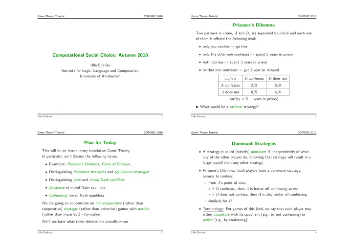
Prisoner’s Dilemma

Two partners in crime, A and B, are separated by police and each one

• f them is offered the following deal:
• only you confess ❀ go free
• only the other one confesses ❀ spend 5 years in prison
• both confess ❀ spend 3 years in prison
• neither one confesses ❀ get 1 year on remand

uA/uB B confesses B does not A confesses 2/2 5/0 A does not 0/5 4/4 (utility = 5 − years in prison) ◮ What would be a rational strategy?

Ulle Endriss 3 Game Theory Tutorial COMSOC 2010

Dominant Strategies

• A strategy is called (strictly) dominant if, independently of what

any of the other players do, following that strategy will result in a larger payoff than any other strategy.

• Prisoner’s Dilemma: both players have a dominant strategy,

namely to confess: – from A’s point of view: ∗ if B confesses, then A is better off confessing as well ∗ if B does not confess, then A is also better off confessing – similarly for B

• Terminology: For games of this kind, we say that each player may

either cooperate with its opponent (e.g., by not confessing) or defect (e.g., by confessing).

Ulle Endriss 4

Game Theory Tutorial COMSOC 2010

Battle of the Sexes

Ann (A) and Bob (B) have different preferences as to what to do on a Saturday night . . . uA/uB Bob: theatre Bob: football Ann: theatre 2/1 0/0 Ann: football 0/0 1/2 Does Ann have a dominant strategy?

Ulle Endriss 5 Game Theory Tutorial COMSOC 2010

Nash Equilibria

• A Nash equilibrium is a set of strategies, one for each player, such

that no player can improve her payoff by unilaterally deviating from her assigned strategy (❀ John F. Nash, Nobel Prize in Economic Sciences in 1994; Academy Award in 2001).

• Battle of the Sexes: two Nash equilibria

– Both Ann and Bob go to the theatre. – Both Ann and Bob go to see the football match.

• In cases where there are no dominant strategies, a set of

equilibrium strategies is the next best thing.

• Discussion: Games with a Nash equilibrium are nice, because you

do not need to keep your strategy secret and you do not need to waste resources trying to find out about other players’ strategies. Naturally, a unique equilibrium is better.

Ulle Endriss 6 Game Theory Tutorial COMSOC 2010

Back to the Prisoner’s Dilemma

• Unique Nash equilibrium, namely when both players confess:

– if A changes strategy unilaterally, she will do worse – if B changes strategy unilaterally, she will also do worse

• Discussion: Our analysis shows that it would be rational to
• confess. But this seems counter-intuitive, because both players

would be better off if both of them were to remain silent.

• So there’s a conflict: the stable solution of the equilibrium is not

efficient, because the outcome is not Pareto optimal.

• Iterated Prisoner’s Dilemma:

– In each round, each player can either cooperate or defect. – Because the other player could retaliate in the next round, it is rational to cooperate. – But it does not work if the number of rounds is fixed . . .

Ulle Endriss 7 Game Theory Tutorial COMSOC 2010

Game of Chicken

James and Marlon are driving their cars towards each other at top

• speed. Whoever swerves to the right first is a “chicken”.

uJ/uM M drives on M turns J drives on 0/0 8/1 J turns 1/8 5/5 Dominant strategies? Nash equilibria?

Ulle Endriss 8

Game Theory Tutorial COMSOC 2010

Analysing the Game of Chicken

• No dominant strategy (best move depends on the other player)
• Two Nash equilibria:

– James drives on and Marlon turns ∗ if James deviates (and turns), he will be worse off ∗ if Marlon deviates (and drives on), he will be worse off – Marlon drives on and James turns (similar argument)

• If you have reason to believe your opponent will turn, then you

should drive on. If you have reason to believe your opponent will drive on, then you should turn.

Ulle Endriss 9 Game Theory Tutorial COMSOC 2010

How many Nash equilibria?

Keep in mind that the first player chooses the row (T/B) and the second player chooses the column (L/R) . . . L R T 2/2 2/1 B 1/3 3/2 L R T 2/2 2/2 B 2/2 2/2 L R T 1/2 2/1 B 2/1 1/2

Ulle Endriss 10 Game Theory Tutorial COMSOC 2010

Notation and Formal Definition

A strategic game consists of a set of players, a set of actions for each player, and a preference relation over action profiles.

• Players: i ∈ {1, . . . , n}
• Actions: each player i has a set Ai of possible actions
• Action profiles: a = (a1, a2, . . . , an) for players 1, . . . , n
• Preferences: represented by utilities ui : A1 × · · · × An → R

Write (a−i, a′

i) for the action profile that is like a, except that player i

chooses a′

i rather than ai.

Then a (pure) Nash equilibrium is an action profile a such that ui(a) ≥ ui(a−i, a′

i) for every player i and every action a′ i of player i. Ulle Endriss 11 Game Theory Tutorial COMSOC 2010

Remarks

• There are games that have no (pure) Nash equilibrium.
• Observe that while we use utilities for ease of presentation, only
• rdinal preferences matter (cardinal intensities are irrelevant).
• Here we only model one-off decisions. In some applications,

however, it seems more likely that following a given protocol requires taking a sequence of decisions. But we can map an agent’s decision making capability to a single strategy encoding what the agent would do in any given situation. Hence, the game theoretical-models do apply here as well (see also so-called extensive games).

Ulle Endriss 12

Game Theory Tutorial COMSOC 2010

Competition

Suppose a newspaper announces the following competition: ◮ Every reader may submit a (rational) number between 0 and 100. The winner is the player whose number is closest to two thirds of the mean of all submissions (in case of a tie, the prize money is split equally amongst those with the best guesses). What number would you submit (and why)?

• A. Bosch-Dom`

enech, J.G. Montalvo, R. Nagel, and A. Satorra. One, Two, (Three), Infinity, . . . : Newspaper and Lab Beauty-Contest Experiments. American Eco- nomic Review, 92(5):1687–1701, 2002.

Ulle Endriss 13 Game Theory Tutorial COMSOC 2010

Exercises

• Does the newspaper game have a Nash equilibrium?

If yes, what is it?

• What changes with respect to Nash equilibria if players can only

choose integers?

• What changes if players can only choose integers and the mean is

being multiplied by

9 10 rather than 2 3? Ulle Endriss 14 Game Theory Tutorial COMSOC 2010

A Game without Nash Equilibria

Recall that the following game does not have a Nash equilibrium: L R T 1/2 2/1 B 2/1 1/2 Whichever action the row player chooses, the column player can react in such a way that the row player would have rather chosen the other

• way. And so on . . .

◮ Idea: Use a probability distribution over all possible actions as your strategy instead.

Ulle Endriss 15 Game Theory Tutorial COMSOC 2010

Mixed Strategies

A mixed strategy pi of a player i is a probability distribution over the actions Ai available to i. Example: Suppose player 1 has three actions: T, M and B; and suppose their order is clear from the context. Then the mixed strategy to play T with probability 1

2, M with probability 1 6, and B with

probability 1

3, is written as p1 = ( 1 2, 1 6, 1 3).

The expected payoff of player i for a profile p of mixed strategies: Ei(p) =

• a∈A1×···×An
• sum over all

action profiles a ( payoff for a ui(a) ×

• i∈{1,...,n}

pi(ai)

• probability of

choosing a )

Ulle Endriss 16

Game Theory Tutorial COMSOC 2010

Discussion

• Earlier, the numbers in a game matrix represented ordinal
• preferences. In particular, many different sets of numbers would

represent the same preference relation.

• Ordinal preferences alone don’t allow us to compare “lotteries”:

I like appeltaart more than I like bitterballen more than I like those broodjes they sell at the cantine . . . but this is not enough information to compare bitterballen with a 50-50 chance to win either an appeltaart or a broodje.

• So in the context of mixed strategies, we take the numbers to

represent utility functions over deterministic outcomes; and we assume that the preferences of players over alternative mixed strategy profiles are representable by the expected payoffs wrt. these utility functions.

Ulle Endriss 17 Game Theory Tutorial COMSOC 2010

Mixed Nash Equilibrium

Write (p−i, p′

i) for the mixed strategy profile that is like p, except that

player i chooses p′

i rather than pi.

A mixed Nash equilibrium is a mixed strategy profile p such that Ei(p) ≥ Ei(p−i, p′

i) for every player i and every possible mixed

strategy p′

i for i.

Informally: A mixed Nash equilibrium is a set of mixed strategies, one for each player, so that no player has an incentive to unilaterally deviate from their assigned strategy.

Ulle Endriss 18 Game Theory Tutorial COMSOC 2010

Example

Recall our game without a (pure) Nash equilibrium: L R T 1/2 2/1 B 2/1 1/2 For this particular example, guessing the probabilities for a mixed Nash equilibrium is easy:

• The row player should play T and B with probability 1

2 each.

• The column player should play L and R with probab. 1

2 each.

Given the assigned strategy of the column player, the row player has no incentive to deviate (expected payoff is 1.5 for either one of the two pure strategies), and vice versa.

Ulle Endriss 19 Game Theory Tutorial COMSOC 2010

Existence of Mixed Equilibria

We are not going to prove this central result here: Theorem 1 (Nash, 1950) Every finite strategic game has got at least one mixed Nash equilibrium.

J.F. Nash. Equilibrium Points in n-Person Games. Proc. National Academy of Sciences of the United States of America, 36:48–49, 1950.

Ulle Endriss 20

Game Theory Tutorial COMSOC 2010

Computing Mixed Nash Equilibria

Recall the Game of Chicken, now in more abstract a form . . . L R T 0/0 8/1 B 1/8 5/5 We’ve already seen that this game has two pure Nash equilibria. Does it also have a (truly) mixed equilibrium? How can we compute such an equilibrium? ◮ Note that (( 1

2, 1 2), ( 1 2, 1 2)) does not work this time (why?). Ulle Endriss 21 Game Theory Tutorial COMSOC 2010

Best Response of Player 1

Let p (q) be the probability that player 1 (player 2) plays T (L): L R T 0/0 8/1 B 1/8 5/5 L R T p · q p · (1 − q) B (1 − p) · q (1 − p) · (1 − q) Expected payoff for 1 playing T given q: E1(T, q) = q · 0 + (1 − q) · 8 Expected payoff for 1 playing B given q: E1(B, q) = q · 1 + (1 − q) · 5 Solving E1(T, q) ≥ E1(B, q) yields q ≤ 3

4.

◮ The best response p of player 1 is given by the following function: p ∈ best1(q) =        {1} if E1(T, q) > E1(B, q), i.e. if q < 3

4

[0, 1] if E1(T, q) = E1(B, q), i.e. if q = 3

4

{0} if E1(T, q) < E1(B, q), i.e. if q > 3

4 Ulle Endriss 22 Game Theory Tutorial COMSOC 2010

Computing Mixed Nash Equlibria (cont.)

The same kind of reasoning can be used to compute the best response function of player 2 as well (payoffs happen to be symmetric here): q ∈ best2(p) =        {1} if E2(L, p) > E2(R, p), i.e. if p < 3

4

[0, 1] if E2(L, p) = E2(R, p), i.e. if p = 3

4

{0} if E2(L, p) < E2(R, p), i.e. if p > 3

4

Each intersection of the two curves corresponds to a mixed Nash equilibrium ((p, 1 − p), (q, 1 − q)): ((1, 0),(0, 1)): player 1 plays T and player 2 plays R [pure] ((0, 1),(1, 0)): player 1 plays B and player 2 plays L [pure] (( 3

4, 1 4),( 3 4, 1 4)):

player 1 (2) plays T (L) with probability 3

4 Ulle Endriss 23 Game Theory Tutorial COMSOC 2010

Complexity of Computing Nash Equilibria

We have just seen a general method for computing all mixed Nash equilibria for a given two-player game with two actions each. In general, computing Nash equilibria is a very difficult problem. How difficult exactly has been an open question for some time. According to Papadimitriou (2001), “. . . [this] is a most fundamental computational problem whose complexity is wide open.” It was known to be “between” P and NP for some time: having guaranteed existence would be untypical for NP-hard problems, but no polynomial algorithm was known either. It has been shown to be PPAD-complete in 2005 (various papers by Goldberg, Papadimitriou, Daskalakis, Chen, Deng) . . .

C.H. Papadimitriou. Algorithms, Games, and the Internet. Proc. STOC-2001.

Ulle Endriss 24

Game Theory Tutorial COMSOC 2010

Summary

This has been an introduction to Game Theory. You should now know about dominant strategies and both pure and mixed equilibrium

• strategies. You should also be able to compute the mixed Nash

equilibria of a simple game.

• We’ve covered non-cooperative rather than cooperative games.

– Cooperative game theory studies competition amongst coalitions of players rather than amongst individuals . . .

• We’ve covered strategic rather than extensive games.

– Extensive games model interactions as trees . . .

• We’ve covered games with perfect information.

– Games with imperfect information model situations where the players do not know each others’ preferences . . .

Ulle Endriss 25 Game Theory Tutorial COMSOC 2010

References

What we have discussed today would be covered by most textbooks on game theory, including these:

• M.J. Osborne. An Introduction to Game Theory. Oxford

University Press, 2004.

• M.J. Osborne and A. Rubinstein. A Course in Game Theory. MIT

Press, 1994.

• R.B. Myerson. Game Theory: Analysis of Conflict. Harvard

University Press, 1991.

• K. Binmore. Fun and Games. Heath, 1992.

The book by Osborne is the most introductory of these, and it has been my main reference for the preparation of these slides.

Ulle Endriss 26