Priority Queues Given x and y , is x less than, equal to, or greater - PDF document

1/31/2016 A new ADT: Priority Queue • A priority queue holds compare-able data (totally ordered) – Like dictionaries with ordered keys, we need to compare CSE373: Data Structures and Algorithms items Priority Queues • Given x and y , is x less than, equal to, or greater than y • Meaning of the ordering can depend on your data and Binary Heaps – Integers are comparable, so we’ll use them in examples • But the priority queue ADT is much more general Steve Tanimoto • Typically two fields, the priority and the data Winter 2016 This lecture material represents the work of multiple instructors at the University of Washington. Thank you to all who have contributed! 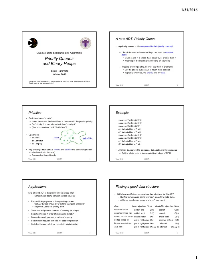Winter 2016 CSE 373 2 Priorities Example • Each item has a “priority” insert x1 with priority 5 – In our examples, the lesser item is the one with the greater priority insert x2 with priority 3 – So “priority 1” is more important than “priority 4” insert x3 with priority 4 – (Just a convention, think “first is best”) a = deleteMin // x2 b = deleteMin // x3 6 2 • Operations: insert x4 with priority 2 15 23 insert – insert insert x5 with priority 6 12 18 deleteMin 45 3 7 – deleteMin c = deleteMin // x4 – is_empty d = deleteMin // x1 • Key property: deleteMin returns and deletes the item with greatest • Analogy: insert is like enqueue , deleteMin is like dequeue priority (lowest priority value) – But the whole point is to use priorities instead of FIFO – Can resolve ties arbitrarily Winter 2016 CSE 373 3 Winter 2016 CSE 373 4 Applications Finding a good data structure Like all good ADTs, the priority queue arises often • Will show an efficient, non-obvious data structure for this ADT – Sometimes blatant, sometimes less obvious – But first let’s analyze some “obvious” ideas for n data items – All times worst-case; assume arrays “have room” • Run multiple programs in the operating system – “critical” before “interactive” before “compute-intensive” data insert algorithm / time deleteMin algorithm / time – Maybe let users set priority level unsorted array add at end O (1) search O ( n ) • Treat hospital patients in order of severity (or triage) unsorted linked list add at front O (1) search O ( n ) • Select print jobs in order of decreasing length? sorted circular array search / shift O ( n ) move front O (1) • Forward network packets in order of urgency sorted linked list put in right place O ( n ) remove at front O (1) • Select most frequent symbols for data compression binary search tree put in right place O ( n ) leftmost O ( n ) • Sort (first insert all, then repeatedly deleteMin ) AVL tree put in right place O ( log n ) leftmost O ( log n ) Winter 2016 CSE 373 5 Winter 2016 CSE 373 6 1

1/31/2016 More on possibilities Our data structure A binary min-heap (or just binary heap or just heap ) has: • Structure property: A complet e binary tree • One more idea: if priorities are 0, 1, …, k can use an array of k lists • Heap property: The priority of every (non-root) node is less – insert : add to front of list at arr[priority] , O (1) important than the priority of its parent – deleteMin : remove from lowest non-empty list O(k) – Not a binary search tree • We are about to see a data structure called a “binary heap” 10 a heap not a heap 10 – Another binary tree structure with specific properties – O ( log n ) insert and O ( log n ) deleteMin worst-case 20 80 20 80 • Possible because we don’t support unneeded operations; no 40 60 85 99 need to maintain a full sort 30 15 50 700 – Very good constant factors So: – If items arrive in random order, then insert is O (1) on average • Where is the highest-priority item? • Because 75% of nodes in bottom two rows • What is the height of a heap with n items? Winter 2016 CSE 373 7 Winter 2016 CSE 373 8 Operations: basic idea DeleteMin Delete (and later return) value at root node • findMin : return root.data 10 • deleteMin : 1 1. answer = root.data 80 20 2. Move right-most node in last 40 60 85 99 4 3 row to root to restore structure property 50 700 7 5 8 9 3. “Percolate down” to restore heap property 11 9 6 10 Overall strategy: • insert: • Preserve structure property 1. Put new node in next position • Break and restore heap on bottom row to restore structure property property 2. “Percolate up” to restore heap property Winter 2016 CSE 373 9 Winter 2016 CSE 373 10 DeleteMin: Keep the Structure Property DeleteMin: Restore the Heap Property Percolate down: • Keep comparing priority of item with both children • If priority is less important, swap with the most important child and • We now have a “hole” at the root go down one level – Need to fill the hole with another value 4 3 • Done if both children are less important than the item or we’ve reached a leaf node 7 5 8 9 10 • Keep structure property: When we are done, ? 10 the tree will have one less node and must still 3 ? 3 11 9 6 10 be complete 4 3 4 4 8 • Pick the last node on the bottom row of the 7 5 8 9 7 5 8 9 7 5 10 9 tree and move it to the “hole” 4 3 11 9 6 11 9 6 11 9 6 7 5 8 9 Why is this correct? 11 9 6 10 What is the run time? Winter 2016 CSE 373 11 Winter 2016 CSE 373 12 2

1/31/2016 DeleteMin: Run Time Analysis Insert • Run time is O (height of heap) • Add a value to the tree 2 • A heap is a complete binary tree • Afterwards, structure and heap 1 properties must still be correct • Height of a complete binary tree of n nodes? – height =  log 2 ( n )  4 8 7 5 10 9 • Run time of deleteMin is O ( log n ) 11 9 6 CSE 373 Winter 2016 CSE 373 13 Winter 2016 14 Insert: Maintain the Structure Property Insert: Restore the heap property Percolate up: • Put new data in new location • If parent is less important, swap with parent, and continue 2 • Done if parent is more important than item or reached root • There is only one valid tree shape after we add one more node 1 2 1 1 ? 1 • So put our new data there and then 4 8 focus on restoring the heap property 4 8 4 8 2 8 7 5 10 9 7 5 10 9 7 10 9 7 4 10 9 11 9 6 ? ? 11 9 6 11 9 6 5 11 9 6 5 2 2 What is the running time? Like deleteMin , worst-case time proportional to tree height: O (log n ) Winter 2016 CSE 373 15 Winter 2016 CSE 373 16 Efficiently Implementing the Priority Summary Queue ADT • Priority Queue ADT: 6 2 – insert comparable object, By using a special data structure called a binary heap *, we will 15 23 insert 12 18 deleteMin – deleteMin achieve: 45 3 7 • Binary heap data structure: • In-place data representation (no links, no wasted fields). 10 – Complete binary tree • Fast insert and deleteMin operations -- O(log n) 20 80 – Each node has less important 40 60 85 99 • Fast initialization of an n-element priority queue (the priority value than its parent 700 50 buildHeap operation) – O(n) • insert and deleteMin operations = O (height-of-tree)= O ( log n ) – insert : put at new last position in tree and percolate-up – deleteMin : remove root, put last element at root and *Be careful not to confuse the binary heap data structure with other meanings of percolate-down “heap” as in “runtime heap” (a pool of memory locations available for dynamic allocation). Winter 2016 CSE 373 17 Winter 2016 CSE 373 18 3