
SLIDE 1
- R. J. Wilkes
Email: ph116@u.washington.edu
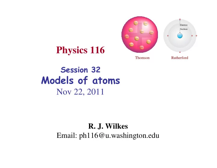
Physics 116
Session 32
Models of atoms
Nov 22, 2011
Thomson Rutherford
Physics 116 Thomson Rutherford Session 32 Models of atoms Nov - - PowerPoint PPT Presentation
Physics 116 Thomson Rutherford Session 32 Models of atoms Nov 22, 2011 R. J. Wilkes Email: ph116@u.washington.edu Announcements Exam 3 next week (Tuesday, 11/29) Usual format and procedures Ill post example questions on the
Thomson Rutherford
afternoon, as usual
Enjoy your holiday weekend!
3
Today
4
– Size of atoms was approximately known from chemistry – He finds: scattering is off a much smaller very dense core (nucleus )
surrounded by negatively charged lightweight electrons
– Atoms have fixed energy states: they cannot “soak up” arbitrary energy – Quanta are emitted when atom “jumps” from high to low E state – Assumed photon’s energy E= hf, as Planck and Einstein suggested – Simple model of electrons orbiting nucleus, and “classical” physics (except for quantized E) gives predictions that match results well (at least, for hydrogen spectrum)
Next topics: atoms, nuclei, radioactivity, subatomic particles
5
Excite a low-pressure sample of noble gas (like neon) with an electric discharge: Pass this light through a slit and prism and you see sharp, separated lines, NOT a continuous rainbow:
Boltzmann’s thermodynamics + Maxwell’s electrodynamics explain only continuous spectra:
wavelength (in Angstroms = 10-10 m) "Holes" in the rainbow?
What causes these sharp lines, in both emission and absorption spectra?
look closely at spectrum of sunlight and you see dark lines in it
6
1. Masses of data collected (“bug collections”) 2. Empirical rules discovered suggesting underlying regularities 3. Rules lead to models of atomic structure 4. Models lead to a refined theory that (eventually) can explain everything – and make predictions of as yet unseen phenomena, to provide a test
– Heat hydrogen in a tube and run through a diffraction grating and you see lines with wavelengths that satisfy the rule (Balmer, 1885) – Outside the visible range, similar series of lines are found, in different EM wavelength regions, named after the rule-finders:
1 λ = R 1 ′ n 2 − 1 n2 ⎛ ⎝ ⎜ ⎞ ⎠ ⎟ , ′ n = 1,2,3K n = ′ n +1
( ),
′ n + 2
( ),
′ n + 3
( )K
R = Rydberg constant
1 λ = R 1 22 − 1 n2 ⎛ ⎝ ⎜ ⎞ ⎠ ⎟ , n = 3,4,5K R = 1.097 ×10⁷ m−1
n’ Series name (range) 1 Lyman (UV) 2 Balmer (visible) 3 Paschen (IR)
negative (q= -e) particles; atoms are larger, and neutral (q= 0)
– perhaps positive charge occupies a blob the size of the atom, and the electrons are like plums in a pudding?
– Alpha-rays (q= + 2e) scatter off atoms as if there were a tiny hard core, like a billiard ball: large scattering angles, sometimes even knocked backwards – Perhaps positive charge occupies only a small volume in the atom, and most of the mass is in this nucleus?
Thomson Rutherford
Rutherford experiment
Radioactive mineral in a lead box with a pinhole Phosphorescent screen Gold foil Beam of “alpha-rays”
Maxwell/Newton physics
1. Electrons are negative particles, occupying circular orbits around a positively charged nucleus (Rutherford model + classical physics) 2. Only certain orbits are allowed: ones where electron’s angular momentum L = integer multiple of hbar (quantized) 3. Electrons do not radiate while in stable circular orbits (contrary to Maxwell!) 4. Radiation occurs only when electrons move between allowed orbits, absorbing or releasing energy (quantum jumps)
– Assumption 1 means electron speed/momentum depends on radius
8
Ln = nh h = h / 2π
( )
mv2 r = ke2 r2 ⇒ v2 = ke2 rm L = mv
mr = nh 2πr
nm
– Assumption 2 defines allowed radii: equate v from assumption 1 with v derived from quantization condition: – All the constants above were known fairly well in 1911: r1= 5.3 x 10⁻¹¹ m – Assumption 4 means allowed radii correspond to energy levels (quantized) – Put in the value of r from above: – Energy released when electron jumps from one n to another:
9
v2 = ke2 rm = Ln mr
n
⎛ ⎝ ⎜ ⎞ ⎠ ⎟
2
= nh 2πr
nm
⎛ ⎝ ⎜ ⎞ ⎠ ⎟
2
⇒ r
n = n2
h2 4π 2mke2 ⎛ ⎝ ⎜ ⎞ ⎠ ⎟ , n = 1,2,3K
E = K +U = mv2 2 − kZe2 r = kZe2 2r − kZe2 r = − 1 2 kZe2 r
(Z=1 for hydrogen)
much energy to extract the electron from the atom
En = − 2π 2mk2e4h2 h2 ⎛ ⎝ ⎜ ⎞ ⎠ ⎟ Z 2 n2 = − 13.6eV
n2 , n = 1,2,3K
∆E ni → n f
2π 2mk2e4 h2 ⎛ ⎝ ⎜ ⎞ ⎠ ⎟ 1 n f
2 − 1
ni
2
⎛ ⎝ ⎜ ⎞ ⎠ ⎟ ∆E = hf = hc λ ⇒ 1 λ = ∆E hc = 2π 2mk2e4 h3c ⎛ ⎝ ⎜ ⎞ ⎠ ⎟ 1 n f
2 − 1
ni
2
⎛ ⎝ ⎜ ⎞ ⎠ ⎟ = 1.097 ×10⁷ m−1
n f
2 − 1
ni
2
⎛ ⎝ ⎜ ⎞ ⎠ ⎟ Bohr explains hydrogen spectra: Lyman series has nf=1, Balmer has nf=2, etc
Rydberg constant !
10
– Electrons like tiny planets orbiting popcorn-ball nucleus at center
– Nucleus is tiny (would be invisible on this picture’s scale) – Particles (protons and electrons) are not really at any point in space – probability distribution describes their location You can observe an electron’s path, but to do so you must knock it out of the atom!
Electron tracks in a cloud chamber (1937)
sciencemuseum.org.uk
11
angular momentum and energy
– Assume e’s have a wave character on the same basis as photons have particle character: – Calculate the wavelengths corresponding to Bohr’s allowed e orbits
p = h λ for photons ⇒ λ = h p for electrons Ln = rnmv = p = mv = h λ ⇒ = for electrons
DeBroglie found that Bohr’s orbit rules corresponded to having circumference of orbit exactly fit m (integer number) wavelengths! Other radii not allowed because overlapping waves “interfere destructively”. Semi-classical picture: related quantum facts to well-known classical phenomena Bohr deBroglie
12
be used to understand subatomic phenomena
– Wave equation defines behavior of a wave function
and momentum at any time:
wave function = Ψ(x, p , t) …this means Ψ depends on x, p and time – Mathematical form ensures proper wavelike behavior of particles – Interference effects (constructive and destructive) are possible!
– Wave function contains all information about quantum system (particle, or atom, or nucleus, or whatever)
answered by solving the wave equation for a completely-specified wave function has no physical meaning !
13
– We can measure E field amplitude (volts per meter) with special hardware – More commonly, we measure intensity of light (energy/sec)
(this gave Schrödinger a hint! )
– Here is the equation describing waves on a string: – Here is the wave equation governing E-M waves: – Here is Schrödinger’s wave equation Notice a difference: Schrödinger’s is “first order” equation (no squares)
2 2 2 2 2
( , ) 1 at position x f x t vertical displacement f along string speed on s f v wave x t g t r n v i = ⎧ ∂ ∂ = ⎨ = ∂ ∂ ⎩
2 2 2 2 2
( , ) 1 at position x E x t E E E c ligh spe t x c t ed = ⎧ ∂ ∂ = ⎨ = ∂ ∂ ⎩
2
( , ) ' ( ) 2 / 2 x t Schrodinger wave function Planck s consta "h - bar nt " x m t π Ψ = ⎧ ∂Ψ − ∂Ψ = ⎨ = ∂ ∂ ⎩ h h
These are called differential equations: they involve partial derivatives (concept from calculus: derivative = rate of change)
14
– Wave function Ψ is not a physical quantity like momentum or E
– Wave function squared gives probability of finding particle at position x (or with momentum p)
0.1 0.2 0.3 0.4 0.5
8 18 28 X Psi
0.05 0.1 0.15 0.2
8 18 28 X Psi2 Wavefunction Ψ(x) (has no units!)
Probability of finding particle described by Ψ(x) at position x: P(x) = Ψ2