Performance Analysis of Coarray-Based MUSIC and the Cram er-Rao - - PowerPoint PPT Presentation

CSSIP

Performance Analysis of Coarray-Based MUSIC and the Cram´ er-Rao Bound

Mianzhi Wang, Zhen Zhang, and Arye Nehorai Preston M. Green Department of Electrical & Systems Engineering Washington University in St. Louis March 8, 2017

1

CSSIP

Outline

• Measurement model and coarray-based MUSIC
• Mean-square error of coarray-based MUSIC
• Cram´

er-Rao bound

• Conclusions and future work

2

CSSIP

Notations

AH = Hermitian transpose of A A∗ = Conjugate of A A† = (AHA)−1AH, pseudo inverse of A ΠA = AA†, projection matrix onto the range space of A Π⊥

A = I − AA†, projection matrix onto the null space of A

⊗ = Kronecker Product ⊙ = Khatri-Rao Product vec(A) = Vectorization of A R(A) = Real part of A I(A) = Imaginary part ofA

3

CSSIP

Measurement Model

• We consider a far-field narrow-band measurement model of sparse linear arrays:

y(t) = A(θ)x(t) + n(t), (1) where A = [a(θ1) a(θ2) · · · a(θK)], with the i-th element of a(θk) being ej ¯

diφk,

¯ di = di/d0, φk = (2πd0 sin θk)/λ, and λ denotes the wavelength.

ULA: Co-prime array: Nested array: MRA: Sparse linear arrays Figure 1: Examples of sparse linear arrays.

4

CSSIP

Measurement Model (cont.)

• We consider the stochastic (unconditional) model [1], where the sources signals

are assumed random and unknown.

• Assumptions:
• 1. The source signals are temporally and spatially uncorrelated.
• 2. The noise is temporally and spatially uncorrelated Gaussian that is also

uncorrelated from the source signals.

• 3. The K DOAs are distinct.
• The sample covariance matrix is given by

R = E[yyH] = AP AH + σ2

nI,

(2) where P = diag(p1, p2, . . . , pL) is the source covariance matrix.

5

CSSIP

Coarray-based MUSIC

• Vectorizing R leads to

r = vec R = Adp + σ2

ni,

(3) where p = [p1, p2, . . . , pK]T , i = vec(I), and Ad = A∗ ⊙ A =

       

ej( ¯

d1− ¯ d1)φ1

· · · ej( ¯

d1− ¯ d1)φk

. . . ... . . . ej( ¯

dm− ¯ dn)φ1

· · · ej( ¯

dm− ¯ dn)φk

. . . ... . . . ej( ¯

dM − ¯ dM )φ1

· · · ej( ¯

dM − ¯ dM )φk

       

. (4)

• Observation: Ad embeds a steering matrix of an difference coarray whose sensor

locations are given by Dco = {dm − dn|1 ≤ m, n ≤ M}. ⇒ We can construct a virtual ULA model from (3).

6

CSSIP

Coarray-based MUSIC (cont.)

Example 1. An illustration of the relationship between the physical array and the

difference coarray.

(a) d0 (b) (c) −Mvd0 Mvd0 ULA of 2Mv − 1 sensors 1st subarray of size Mv

Figure 2: A co-prime array with sensors located at [0, 2, 3, 4, 6, 9]λ/2 and its coarray: (a) physical array, (b) coarray, (c) virtual ULA part of the coarray.

7

CSSIP

Coarray-based MUSIC (cont.)

Definition 1. The array weight function [2] ω(n) : Z → Z is defined by

ω(l) = |{(m, n)| ¯ dm − ¯ dn = l}|, where |A| denotes the cardinality of the set A.

Definition 2. Let 2Mv − 1 denote the size of the central virtual ULA. We introduce

the transform matrix [3] F as a real matrix of size (2Mv − 1) × M 2, whose elements are defined by Fm,p+(q−1)M =

• 1

ω(m−Mv)

, ¯ dp − ¯ dq = m − Mv, , otherwise, (5) for m = 1, 2, . . . , Mv, p = 1, 2, . . . , M, q = 1, 2, . . . , M. ⇒ We can express the measurement vector of the virtual ULA model by z = F r = Acp + σ2

nF i.

(6)

8

CSSIP

Coarray-based MUSIC (cont.)

• To construct the augmented sample covariance matrix, the virtual ULA is divided

into Mv overlapping subarrays of size Mv [2], [4].

• We denote the output of the i-th subarray by zi = Γiz for i = 1, 2, . . . , Mv,

where Γi = [0Mv×(i−1) IMv×Mv 0Mv×(Mv−i)].

−Mvd0 Mvd0 ULA of 2Mv − 1 sensors 1st subarray 2nd subarray ... Mv-th subarray

Figure 3: Mv overlapping subarrays.

9

CSSIP

Coarray-based MUSIC (cont.)

• We can then construct an augmented covariance matrix Rv from zi to provide

enhanced degrees of freedom and apply MUSIC to Rv.

• Two commonly used methods:

◮ MUSIC with directly augmented covariance matrix (DA-MUSIC) [4]:

Rv1 = [zMv zMv−1 · · · z1]. (7)

◮ MUSIC with spatially smoothed covariance matrix (SS-MUSIC) [2]:

Rv2 = 1 Mv

Mv

• i=1

zizH

i .

(8)

• Rv1 and Rv2 are related via the following equality [2]:

Rv2 = 1 Mv R2

v1 =

1 Mv (AvP AH

v + σ2 nI)2,

(9) where Av corresponds to the steering matrix of a ULA whose sensors are located at [0, 1, . . . , Mv − 1]d0.

10

CSSIP

Outline

• Measurement model and coarray-based MUSIC
• Mean-square error of coarray-based MUSIC
• Cram´

er-Rao bound

• Conclusions and future work

11

CSSIP

Mean-Square Error of Coarray-Based MUSIC

We derive the closed-form MSE expressions for DA-MUSIC and SS-MUSIC:

Theorem 1. Let ˆ

θ(DA)

k

and ˆ θ(SS)

k

denote the estimated values of θk using DA-MUSIC and SS-MUSIC, respectively. Let ∆r = vec( ˆ R − R). Then [3] ˆ θ(DA)

k

− θk . = ˆ θ(SS)

k

− θk . = − λ 2πd0pk cos θk I(ξT ∆r) βH

k βk

, (10) where . = denotes asymptotic equality (first-order) and ξk = F T ΓT (βk ⊗ αk), αT

k = −eT k A† v,

βk = Π⊥

AvDav(θk).

Γ = [ΓT

Mv ΓT Mv−1 · · · ΓT 1 ]T ,

D = diag(0, 1, . . . , Mv),

Theorem 2. The asymptotic MSE expressions of DA-MUSIC and SS-MUSIC have

the same form. Denote the asymptotic MSE of the k-th DOA by ǫ(θk). We have [3]: ǫ(θk) = λ2 4π2Nd2

0p2 k cos2 θk

ξH

k (R ⊗ RT )ξk

βk4

2

, ∀k ∈ {1, 2, . . . , K}. (11)

12

CSSIP

Mean-Square Error of Coarray-Based MUSIC (cont.)

Theorem 1 and Theorem 2 have the following implications:

• DA-MUSIC and SS-MUSIC have the same asymptotic MSE, and they are both

asymptotically unbiased.

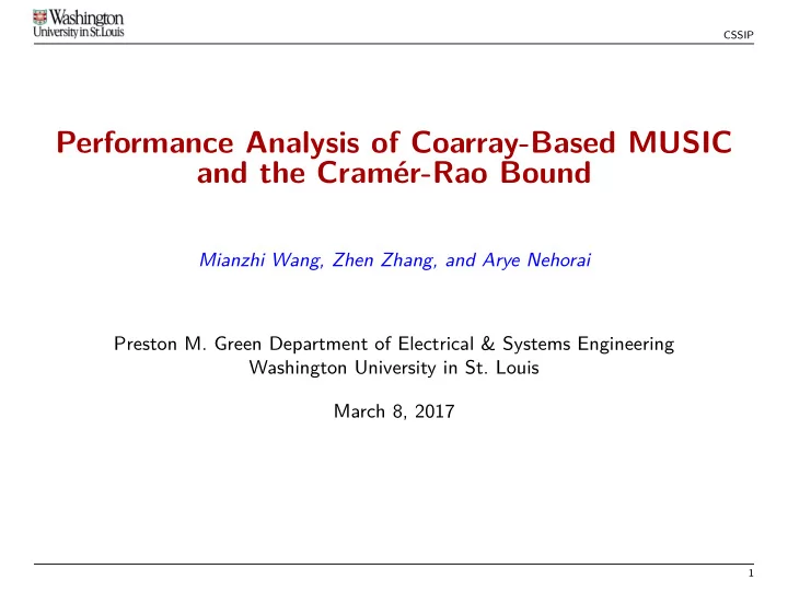
• ǫ(θk) depends on both the physical array geometry and the coarray geometry (as

illustrated in Fig. 4).

• 10

10 20

SNR (dB)

0.08 0.1 0.12 0.14 0.16

RMSE (deg)

Nested (5, 6) Nested (2, 12) Nested (3, 9) Nested (1, 18)

• 10

10 20

SNR (dB)

0.15 0.2 0.25

RMSE (deg)

Nested (5, 6) Nested (2, 12) Nested (3, 9) Nested (1, 18)

Figure 4: RMSE vs. SNR for four different nested array configurations. The four arrays share the same virtual ULA. Left: K = 8. Right: K = 20.

13

CSSIP

Mean-Square Error of Coarray-Based MUSIC (cont.)

Corollary 1. Assume all sources have the same power p. Let SNR = p/σ2

n denote

the common SNR. Then ǫ(θk) decreases monotonically as SNR increases, and lim

SNR→∞ ǫ(θk) =

λ2 4π2Nd2

0p2 k cos2 θk

ξH

k (A ⊗ A∗)2 2

βk4

2

. (12) Specifically,

• 1. when K = 1, the above expression is exactly zero;
• 2. when K ≥ M the above expression is strictly greater than zero.

Implication:

Corollary 1 analytically explains the “saturation” behavior of SS-MUSIC in high SNR regions observed in previous studies.

14

CSSIP

Mean-Square Error of Coarray-Based MUSIC (cont.)

MSE vs. number of sensors:

4 14 50

M

10-6 10-4 10-2

MSE (deg2)

Coprime Nested O(M −4.4)

(a) K = 1 4 14 50

M

10-6 10-4 10-2

MSE (deg2)

Coprime Nested O(M −4.4)

(b) K = 3 Figure 5: MSE vs. number of sensors. SNR = 0dB, and N = 1000. The solid lines denote analytical results, while crosses denote numerical results. A dashed black trend line is included for comparison. The co-prime arrays were generated by the co-prime pairs (m, m + 1), and the nested arrays were generated by the parameter pairs (m + 1, m), where we varied m from 2 to 12.

Observation: the MSE of coarray-based MUSIC decreases faster than O(M −3), the asymptotic MSE of classical MUSIC for ULAs when M → ∞.

15

CSSIP

Mean-Square Error of Coarray-Based MUSIC (cont.)

Resolution analysis: The analytical resolution limit is determined by

• ǫ(θ − ∆θ/2) +
• ǫ(θ − ∆θ/2) ≥ ∆θ

(13)

Figure 6: Resolution probability of different arrays for different N with SNR fixed to 0dB, obtained from 500

• trials. The red dashed line is the analytical resolution limit.

Figure 7: Resolution probability of different arrays for different SNRs with N = 1000, obtained from 500 trials. The red dashed line is the analytical resolution limit.

Observation: our analytical expression predict the resolution limit well.

16

CSSIP

Outline

• Measurement model and coarray-based MUSIC
• Mean-square error of coarray-based MUSIC
• Cram´

er-Rao bound

• Conclusions and future work

17

CSSIP

Cram´ er-Rao Bound

• The CRB of the DOAs for general sparse linear arrays with under the assumption
• f uncorrelated sources is given by [3], [5], [6]:

CRBθ = 1 N (M H

θ Π⊥ MsMθ)−1,

(14) where Mθ = (RT ⊗ R)−1/2 ˙ AdP , (15a) Ms = (RT ⊗ R)−1/2 Ad i , (15b) ˙ Ad = ˙ A∗ ⊙ A + A∗ ⊙ ˙ A, (15c) ˙ A = [∂a(θ1)/∂θ1, · · · , ∂a(θK)/∂θK], (15d) and Ad, i follow the same definitions as in (3).

• The CRB can be valid even if the number of sources exceeds the number of
• sensors. This is because the invertibility of the FIM depends on the coarray

structure, which appears in [ ˙ AdP Ad i]. The can remain full column rank of [ ˙ AdP Ad i] even if K ≥ M.

18

CSSIP

Cram´ er-Rao Bound (cont.)

Proposition 1. Assume all sources have the same power p, and [ ˙

AdP Ad i is full column rank. Let SNR = p/σ2

• n. Then
• 1. If K < M, and limSNR→∞ CRBθ exists, it is zero under mild conditions;
• 2. If K ≥ M, and limSNR→∞ CRBθ exists, it is positive definite when K ≥ M.

Implications:

• When K < M, the CRB approaches zero as SNR → ∞, which is similar to the

ULA case.

• When K ≥ M, the CRB exhibits a different behavior by converging to a strictly

positive definite matrix. This puts an strictly positive lower bound on the MSE of all unbiased estimators.

• Recall that in Corollary 1, when K ≥ M, ǫ(θk) converges to a positive constant

as SNR → ∞. We now know that this is not because of the choice of the algorithms, but the asymptotic error ǫ(θk) > 0 is inherent in the model as shown by the CRB.

19

CSSIP

Cram´ er-Rao Bound (cont.)

Theorem 3. Assume that all sources share the same power. For co-prime arrays

generated with co-prime pair (Q, Q + 1), or nested arrays generated with parameter pair (Q, Q), if we fix K ≪ Q, then as Q → ∞, the CRB can decrease at a rate of O(Q−5).

Observation:

For ULAs, the CRB decreases at a rate of O(M −3) as the number of sensors M → ∞ [7]. Theorem 3 implies that co-prime and nested arrays can achieve the same performance as ULAs with fewer sensors. This behavior can be attributed to the fact that a M-sensor co-prime array or nested array has a much larger aperture than a M-sensor ULA.

20

CSSIP

Cram´ er-Rao Bound (cont.)

CRB vs. number of sensors for co-prime and nested arrays:

100 101 102

M

10-9 10-5 10-1

CRB (deg2)

Coprime Nested O(M −5) (a) K = 1

100 101 102

M

10-9 10-5 10-1

CRB (deg2)

Coprime Nested O(M −5) (b) K = 3 Figure 8: CRB vs. number of sensors. SNR = 0dB, and N = 1000. A dashed black trend line is included for comparison.

Observation: the CRB precisely follows the trend line of O(M −5) for large M.

21

CSSIP

Conclusions and Future Work

Conclusions

• DA-MUSIC and SS-MUSIC have the same asymptotic MSE.
• When there are more sources than sensors, both the MSE of DA-MUSIC

(SS-MUSIC) and the CRB are strictly non-zero as SNR → ∞.

• The CRB for co-prime and nested arrays with O(M) sensors can decrease at a

rate of O(M −5), which analytically shows that such arrays can achieve similar performance to ULAs with fewer sensors.

Future work:

• Analytical resolution analysis
• Sensitivity analysis against model errors
• Optimal array geometry design

22

CSSIP

References I

• P. Stoica and A. Nehorai, “Performance study of conditional and unconditional

direction-of-arrival estimation,” IEEE Transactions on Acoustics, Speech and Signal Processing, vol. 38, no. 10, pp. 1783–1795, Oct. 1990, issn: 0096-3518. doi: 10.1109/29.60109.

• P. Pal and P. Vaidyanathan, “Nested arrays: A novel approach to array

processing with enhanced degrees of freedom,” IEEE Transactions on Signal Processing, vol. 58, no. 8, pp. 4167–4181, Aug. 2010, issn: 1053-587X. doi: 10.1109/TSP.2010.2049264.

• M. Wang and A. Nehorai, “Coarrays, MUSIC, and the Cram´

e Rao Bound,” IEEE Transactions on Signal Processing, vol. 65, no. 4, pp. 933–946, Feb. 2017, issn: 1053-587X. doi: 10.1109/TSP.2016.2626255. C.-L. Liu and P. Vaidyanathan, “Remarks on the spatial smoothing step in coarray MUSIC,” IEEE Signal Processing Letters, vol. 22, no. 9, Sep. 2015, issn: 1070-9908. doi: 10.1109/LSP.2015.2409153.

23

CSSIP

References II

C.-L. Liu and P. P. Vaidyanathan, “Cram´ er Rao bounds for coprime and other sparse arrays, which find more sources than sensors,” Digital Signal Processing,

• no. 61, pp. 43–61, Feb. 2017, issn: 1051-2004. doi:

10.1016/j.dsp.2016.04.011.

• A. Koochakzadeh and P. Pal, “Cram´

er Rao bounds for underdetermined source localization,” IEEE Signal Processing Letters, vol. 23, no. 7, pp. 919–923, Jul. 2016, issn: 1070-9908. doi: 10.1109/LSP.2016.2569504.

• P. Stoica and A. Nehorai, “MUSIC, maximum likelihood, and Cramer-Rao

bound,” IEEE Transactions on Acoustics, Speech and Signal Processing, vol. 37,

• no. 5, pp. 720–741, May 1989, issn: 0096-3518. doi: 10.1109/29.17564.

24

CSSIP

Questions?

25