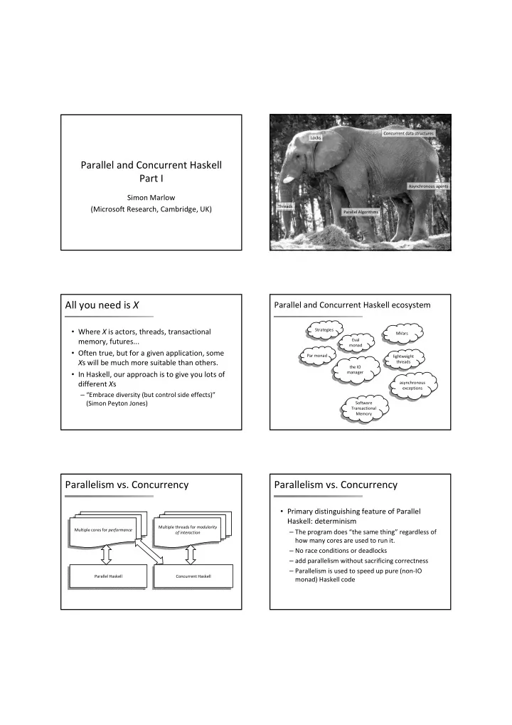
Parallel and Concurrent Haskell Part I Asynchronous agents Simon - PDF document

Concurrent data structures Locks Parallel and Concurrent Haskell Part I Asynchronous agents Simon Marlow Threads (Microsoft Research, Cambridge, UK) Parallel Algorithms All you need is X Parallel and Concurrent Haskell ecosystem Strategies • Where X is actors, threads, transactional MVars memory, futures... Eval monad • Often true, but for a given application, some Par monad lightweight X s will be much more suitable than others. threads the IO • In Haskell, our approach is to give you lots of manager different X s asynchronous exceptions – “Embrace diversity (but control side effects)” (Simon Peyton Jones) Software Transactional Memory Parallelism vs. Concurrency Parallelism vs. Concurrency • Primary distinguishing feature of Parallel Haskell: determinism Multiple threads for modularity Multiple cores for performance – The program does “the same thing” regardless of of interaction how many cores are used to run it. – No race conditions or deadlocks – add parallelism without sacrificing correctness – Parallelism is used to speed up pure (non ‐ IO Parallel Haskell Concurrent Haskell monad) Haskell code

Parallelism vs. Concurrency I. Parallel Haskell • In this part of the course, you will learn how to: • Primary distinguishing feature of Concurrent – Do basic parallelism: Haskell: threads of control • compile and run a Haskell program, and measure its performance – Concurrent programming is done in the IO monad • parallelise a simple Haskell program (a Sudoku solver) • use ThreadScope to profile parallel execution • because threads have effects • do dynamic rather than static partitioning • effects from multiple threads are interleaved • measure parallel speedup nondeterministically at runtime. – use Amdahl’s law to calculate possible speedup – Work with Evaluation Strategies – Concurrent programming allows programs that • build simple Strategies interact with multiple external agents to be modular • parallelise a data ‐ mining problem: K ‐ Means • the interaction with each agent is programmed separately – Work with the Par Monad • Use the Par monad for expressing dataflow parallelism • Allows programs to be structured as a collection of • Parallelise a type ‐ inference engine interacting agents (actors) Running example: solving Sudoku Solving Sudoku problems – code from the Haskell wiki (brute force search • Sequentially: with some intelligent pruning) – divide the file into lines – can solve all 49,000 problems in 2 mins – call the solver for each line – input: a line of text representing a problem i m por t Sudoku i m por t Cont r ol . Except i on .......2143.......6........2.15..........637...........68...4.....23........7.... i m por t Syst em . Envi r onm ent .......241..8.............3...4..5..7.....1......3.......51.6....2....5..3...7... .......24....1...........8.3.7...1..1..8..5.....2......2.4...6.5...7.3........... m ai n : : I O ( ) m ai n = do [ f ] <- get Ar gs gr i ds <- f m ap l i nes $ r eadFi l e f i m por t Sudoku m apM ( eval uat e . sol ve) gr i ds sol ve : : St r i ng - > M aybe G r i d eval uat e : : a - > I O a Compile the program... Run the program... $ . / sudoku1 sudoku17. 1000. t xt +RTS - s 2, 392, 127, 440 byt es al l ocat ed i n t he heap $ ghc - O 2 sudoku1. hs - r t sopt s [ 1 of 2] Com pi l i ng Sudoku ( Sudoku. hs, Sudoku. o ) 36, 829, 592 byt es copi ed dur i ng G C [ 2 of 2] Com pi l i ng M ai n ( sudoku1. hs, sudoku1. o ) 191, 168 byt es m axi m um r esi dency ( 11 sam pl e( s) ) Li nki ng sudoku1 . . . 82, 256 byt es m axi m um sl op $ 2 M B t ot al m em or y i n use ( 0 M B l ost due t o f r agm ent at i on) G ener at i on 0: 4570 col l ect i ons, 0 par al l el , 0. 14s, 0. 13s el apsed G ener at i on 1: 11 col l ect i ons, 0 par al l el , 0. 00s, 0. 00s el apsed . . . I NI T t i m e 0. 00s ( 0. 00s el apsed) M UT t i m e 2. 92s ( 2. 92s el apsed) G C t i m e 0. 14s ( 0. 14s el apsed) EXI T t i m e 0. 00s ( 0. 00s el apsed) Tot al t i m e 3. 06s ( 3. 06s el apsed) . . .

Now to parallelise it... The Eval monad i m por t Cont r ol . Par al l el . St r at egi es • Doing parallel computation entails specifying dat a Eval a coordination in some way – compute A in i nst ance M onad Eval parallel with B r unEval : : Eval a - > a • This is a constraint on evaluation order r par : : a - > Eval a r seq : : a - > Eval a • But by design, Haskell does not have a • Eval is pure specified evaluation order • Just for expressing sequencing between rpar/rseq – nothing more • So we need to add something to the language • Compositional – larger Eval sequences can be built by to express constraints on evaluation order composing smaller ones using monad combinators • Internal workings of Eval are very simple (see Haskell Symposium 2010 paper) What does rpar actually do? Basic Eval patterns x <- <- r par e par e • To compute a in parallel with b, and return a • rpar creates a spark by writing an entry in the spark pool pair of the results: – rpar is very cheap! (not a thread) Start evaluating do • the spark pool is a circular buffer a in the a’ <- r par a • when a processor has nothing to do, it tries to remove an background b’ <- r seq b entry from its own spark pool, or steal an entry from r et ur n ( a’ , b’ ) another spark pool ( work stealing) Evaluate b, and • alternatively: • when a spark is found, it is evaluated wait for the • The spark pool can be full – watch out for spark overflow! result do a’ <- r par a e b’ <- r seq b r seq a’ r et ur n ( a’ , b’ ) Spark Pool • what is the difference between the two? Parallelising Sudoku But this won’t work... r unEval $ do • Let’s divide the work in two, so we can solve as’ <- r par ( m ap sol ve as) bs’ <- r par ( m ap sol ve bs) each half in parallel: r seq as’ r seq bs’ r et ur n ( ) l et ( as, bs) = spl i t At ( l engt h gr i ds ` di v` 2) gr i ds • rpar evaluates its argument to Weak Head Normal • Now we need something like Form (WHNF) • WTF is WHNF? r unEval $ do as’ <- r par ( m ap sol ve as) – evaluates as far as the first constructor bs’ <- r par ( m ap sol ve bs) – e.g. for a list, we get either [] or (x:xs) r seq as’ r seq bs’ – e.g. WHNF of “map solve (a:as)” would be “solve a : map r et ur n ( ) solve as” • But we want to evaluate the whole list, and the elements

We need ‘deep’ Ok, adding deep r unEval $ do i m por t Cont r ol . DeepSeq as’ <- r par ( deep ( m ap sol ve as) ) deep : : NFDat a a => a - > a bs’ <- r par ( deep ( m ap sol ve bs) ) deep a = deepseq a a r seq as’ r seq bs’ • deep fully evaluates a nested data structure and r et ur n ( ) returns it • Now we just need to evaluate this at the top level in – e.g. a list: the list is fully evaluated, including the elements ‘main’: • uses overloading: the argument must be an instance of NFData eval uat e $ r unEval $ do a <- r par ( deep ( m ap sol ve as) ) – instances for most common types are provided by the . . . library • (normally using the result would be enough to force evaluation, but we’re not using the result here) Let’s try it... Runtime results... $ . / sudoku2 sudoku17. 1000. t xt +RTS - N2 - s • Compile sudoku2 2, 400, 125, 664 byt es al l ocat ed i n t he heap 48, 845, 008 byt es copi ed dur i ng G C – (add ‐ threaded ‐ rtsopts) 2, 617, 120 byt es m axi m um r esi dency ( 7 sam pl e( s) ) 313, 496 byt es m axi m um sl op 9 M B t ot al m em or y i n use ( 0 M B l ost due t o f r agm ent at i on) – run with sudoku17. 1000. t xt +RTS - N2 G ener at i on 0: 2975 col l ect i ons, 2974 par al l el , 1. 04s, 0. 15s el apsed • Take note of the Elapsed Time G ener at i on 1: 7 col l ect i ons, 7 par al l el , 0. 05s, 0. 02s el apsed Par al l el G C wor k bal ance: 1. 52 ( 6087267 / 3999565, i deal 2) SPARKS: 2 ( 1 conver t ed, 0 pr uned) I NI T t i m e 0. 00s ( 0. 00s el apsed) M UT t i m e 2. 21s ( 1. 80s el apsed) G C t i m e 1. 08s ( 0. 17s el apsed) EXI T t i m e 0. 00s ( 0. 00s el apsed) Tot al t i m e 3. 29s ( 1. 97s el apsed) Calculating Speedup Why not 2? • Calculating speedup with 2 processors: • there are two reasons for lack of parallel speedup: – Elapsed time (1 proc) / Elapsed Time (2 procs) – NB. not CPU time (2 procs) / Elapsed (2 procs)! – less than 100% utilisation (some processors idle for part of the time) – NB. compare against sequential program, not – extra overhead in the parallel version parallel program running on 1 proc • Each of these has many possible causes... • Speedup for sudoku2: 3.06/1.97 = 1.55 – not great...