[PPT] - Overview of Linear Prediction Introduction Terms and definitions PowerPoint Presentation

SLIDE 1

Nonstationary Problem Definition Given a segment of a signal {x(n), x(n − 1), . . . , x(n − M)} of a stochastic process estimate x(n − i) for 0 ≤ i ≤ M using the remaining portion of the signal ˆ x(n − i) −

M

k=0

k=i

c∗

k(n)x(n − k)

e(i)(n) x(n − i) − ˆ x(n − i) =

M

k=0

ck

∗(n)x(n − k)

where ci(n) 1

J. McNames

Portland State University ECE 539/639 Linear Prediction

Ver. 1.02

3

Overview of Linear Prediction

Terms and definitions
Nonstationary case
Stationary case
Forward linear prediction
Backward linear prediction
Stationary processes
Exchange matrices
Examples
Properties
J. McNames

Portland State University ECE 539/639 Linear Prediction

Ver. 1.02

1

Change in Notation ˆ x(n − i) −

M

k=0

k=i

c∗

k(n)x(n − k)

e(i)(n)

M

k=0

ck

∗(n)x(n − k)

Note that this is inconsistent with the notation used earlier,

ˆ yo(n) =

M−1

k=0

ho(k)x(n − k) =

M−1

k=0

c∗

k+1x(n − k)

Also the sums have M + 1 terms in them, rather than M terms as

before

Presumably motivated by a simple expression for the error e(i)(n)
J. McNames

Portland State University ECE 539/639 Linear Prediction

Ver. 1.02

4

Introduction

Important for more applications than just prediction
Prominent role in spectral estimation, Kalman filtering, fast

algorithms, etc.

Prediction is equivalent to whitening! (more later)
Clearly many practical applications as well
J. McNames

Portland State University ECE 539/639 Linear Prediction

Ver. 1.02

2

SLIDE 2

Forward and Backward Linear Prediction Estimator and Error ˆ xf(n) = −

M

k=1

a∗

k(n)x(n − k)

= −aH(n)x(n − 1) ˆ xb(n) = −

M−1

k=0

b∗

k(n)x(n − k)

= −bH(n)x(n) ef = x(n) +

M

k=1

a∗

k(n)x(n − k)

= x(n) + aH(n)x(n − 1) eb =

M−1

k=0

b∗

k(n)x(n − k) + x(n − M)

= bH(n)x(n) + x(n − M)

Again, new notation compared to the FIR linear estimation case
I use subscripts for the f instead of superscripts like the text
J. McNames

Portland State University ECE 539/639 Linear Prediction

Ver. 1.02

7

Types of “Prediction” ˆ x(n − i) −

M

k=0

k=i

c∗

k(n)x(n − k)

e(i)(n)

M

k=0

ck

∗(n)x(n − k)

Forward Linear Prediction: i = 0
Backward Linear Prediction: i = M

– Misnomer, but terminology is rooted in the literature

Symmetric Linear Smoother: i = M/2
J. McNames

Portland State University ECE 539/639 Linear Prediction

Ver. 1.02

5

Forward and Backward Linear Prediction Solution Solution is the same as before, but watch the minus signs R(n − 1)ao(n) = −rf(n) R(n)bo(n) = −rb(n) Pf,o(n) = Px(n) + rH

f (n)ao(n)

Pb,o(n) = Px(n − M) + rH

b (n)bo(n)

ˆ xf(n) = −

M

k=1

a∗

k(n)x(n − k)

= −aH(n)x(n − 1) ˆ xb(n) = −

M−1

k=0

b∗

k(n)x(n − k)

= −bH(n)x(n)

J. McNames

Portland State University ECE 539/639 Linear Prediction

Ver. 1.02

8

Linear “Prediction” Notation and Partitions x(n) x(n) x(n − 1) . . . x(n − M + 1)T ¯ x(n)

x(n)

x(n − 1) . . . x(n − M) T =

x(n)

xT(n − 1) T =

xT(n)

x(n − M) T R(n) = E[x(n)xH(n)] ¯ R(n) = E[¯ x(n)¯ xH(n)] Forward and backward linear prediction use specific partitions of the “extended” autocorrelation matrix ¯ R(n)

Px(n)

rH

f (n)

rf(n) R(n − 1)

¯

R(n) R(n) rb(n) rH

b (n)

Px(n − M)

rf(n) = E[x(n − 1)x∗(n)]

rb(n) = E[x(n)x∗(n − M)]

J. McNames

Portland State University ECE 539/639 Linear Prediction

Ver. 1.02

6

SLIDE 3

Exchange Matrix J ⎡ ⎢ ⎢ ⎢ ⎣ . . . 1 . . . . . . ... . . . 1 . . . 1 . . . ⎤ ⎥ ⎥ ⎥ ⎦ JHJ = JJH = I

Counterpart to the identity matrix
When multiplied on the left, flips a vector upside down
When multiplied on the right, flips a vector sideways
Don’t do this in MATLAB—many wasted multiplications by zeros
See fliplr and flipud
J. McNames

Portland State University ECE 539/639 Linear Prediction

Ver. 1.02

11

Stationary Case: Autocorrelation Matrix When the process is stationary, something surprising happens!

¯ R

(M+1)×(M+1) =

rx(0)

rx(1) . . . rx(M − 1) rx(M) r∗

x(1)

rx(0) . . . rx(M − 2) rx(M − 1) . . . . . . ... . . . . . . r∗

x(M − 1)

r∗

x(M − 2)

. . . rx(0) rx(1) r∗

x(M)

r∗

x(M − 1)

. . . r∗

x(1)

rx(0)

r

M×1

rx(1)

rx(2) . . . rx(M)

T

¯ R(n) =

Px(n)

rH

f (n)

rf(n) R(n − 1)

=

R(n) rb(n) rH

b (n)

Px(n − M)

Clearly,

R(n) = R(n − 1) Px(0) = Px(n − M) = rx(0)

J. McNames

Portland State University ECE 539/639 Linear Prediction

Ver. 1.02

9

Forward/Backward Prediction Relationship Rbo = −rb = −Jr Rao = −rf = −r∗ JRao = −Jr∗ JR∗a∗

= −Jr = −rb

JR∗ = RJ R(Ja∗

) = −rb

bo = Ja∗

The BLP parameter vector is the flipped and conjugated FLP

parameter vector!

Useful for estimation: can solve for both and combine them to

reduce variance

Further the prediction errors are the same!

Pf,o = Pb,o = r(0) + rHao = r(0) + rHJbo

J. McNames

Portland State University ECE 539/639 Linear Prediction

Ver. 1.02

12

Stationary Case: Cross-correlation Vector

¯ R

(M+1)×(M+1) =

rx(0)

rx(1) . . . rx(M) r∗

x(1)

rx(0) . . . rx(M − 1) . . . . . . ... . . . r∗

x(M)

r∗

x(M − 1)

. . . rx(0)

r

M×1

rx(1)

rx(2) . . . rx(M)

¯

R =

rx(0)

rH

f

rf R

=
rx(0)

rT r∗ R

¯

R = R rb rH

b

rx(0)

=

R Jr rHJ rx(0)

rf = E[x(n − 1)x∗(n)]

= r∗ rb = E[x(n)x∗(n − M)] = Jr where J is the exchange matrix

J. McNames

Portland State University ECE 539/639 Linear Prediction

Ver. 1.02

10

SLIDE 4

Example 1: Prediction Example

10 20 30 40 50 60 70 80 90 100 −5 5 Sample Time (n) M:25 i:0

NMSE:0.388

Signal + Estimate (scaled) x(n) ˆ x(n + 0)

J. McNames

Portland State University ECE 539/639 Linear Prediction

Ver. 1.02

15

Example 1: MA Process Create a synthetic MA process in MATLAB. Plot the pole-zero and transfer function of the system. Plot the MMSE versus the point being estimated, ˆ x(n − i) −

M

k=0

k=i

c∗

k(n)x(n − k)

for M = 25.

J. McNames

Portland State University ECE 539/639 Linear Prediction

Ver. 1.02

13

Example 1: Prediction Example

10 20 30 40 50 60 70 80 90 100 −5 5 Sample Time (n) M:25 i:13

NMSE:0.168

Signal + Estimate (scaled) x(n) ˆ x(n + 13)

J. McNames

Portland State University ECE 539/639 Linear Prediction

Ver. 1.02

16

Example 1: MMSE Versus Prediction Index i

5 10 15 20 25 0.2 0.4 0.6 0.8 1 Prediction Index (i, Samples) MNMSE Minimum NMSE Estimated MNMSE

J. McNames

Portland State University ECE 539/639 Linear Prediction

Ver. 1.02

14

SLIDE 5

end; end; Po = zeros(M+1,1); X = zeros(N,M+1); Poh = zeros(M+1,1); for id=0:M, R = [Re(1:id ,1:id),Re(1:id ,id+2:end);... Re(id+2:end,1:id),Re(id+2:end,id+2:end)]; d = [Re(1:id,id+1);Re(id+2:end,id+1)]; % Extract i’th column sans the ith row Px = Re(id+1,id+1); co = -inv(R)*d; Po(id+1) = Px + d’*co; X(:,id+1) = filter(-[co(1:id);0;co(id+1:end)],1,x); k = 1:N-(id+1); Poh(id+1) = mean((x(k)-X(k+id,id+1)).^2); end; %================================================ % Plot MMSE Versus Order %================================================ figure; FigureSet(1,’LTX’); h1 = plot3(0:M,Poh/var(x),-1*ones(M+1,1),’ro’); set(h1,’MarkerFaceColor’,’r’); set(h1,’MarkerSize’,6); view(0,90); hold on; h2 = stem(0:M,Po/Px,’k’); set(h2,’MarkerFaceColor’,’k’); set(h2,’MarkerSize’,4); hold off; xlabel(’Prediction Index (i, Samples)’); ylabel(’MNMSE’); box off; xlim([-0.5 M+0.5]); ylim([0 1.05]);

J. McNames

Portland State University ECE 539/639 Linear Prediction

Ver. 1.02

19

Example 1: Prediction Example

10 20 30 40 50 60 70 80 90 100 −5 5 Sample Time (n) M:25 i:25

NMSE:0.388

Signal + Estimate (scaled) x(n) ˆ x(n + 25)

J. McNames

Portland State University ECE 539/639 Linear Prediction

Ver. 1.02

17

AxisLines; AxisSet(8); legend([h1;h2],’Minimum NMSE Estimated’,’MNMSE’); print(’MAExampleMNMSEvi’,’-depsc’); %================================================ % Plot Estimates %================================================ id = [0,round(M/2),M]; for c1=1:length(id), k = 1:N-(id(c1)+1); xh = X(k+id(c1),id(c1)+1); figure; FigureSet(2,’LTX’); h = plot(k,x(k),’b’,k,xh(k),’g’); set(h,’LineWidth’,0.8); set(h,’Marker’,’.’); set(h,’MarkerSize’,8); xlim([0 100]); ylim(std(x)*[-3 3]); AxisLines; xlabel(’Sample Time (n)’); ylabel(’Signal + Estimate (scaled)’); set(get(gca,’Title’),’Interpreter’,’LaTeX’); title(sprintf(’M:%d i:%d $\\widehat{\\mathrm{NMSE}}$:%5.3f’,M,id(c1),mean((x(k)-xh).^2)/var(x(k)))); box off; AxisSet(8); hl = legend(h,’$x(n)$’,sprintf(’$\\hat{x}(n+%d)$’,id(c1))); set(hl,’Interpreter’,’LaTeX’) print(sprintf(’MAExamplePlot%02d’,id(c1)),’-depsc’); end;

J. McNames

Portland State University ECE 539/639 Linear Prediction

Ver. 1.02

20

Example 1: MATLAB Code

clear all; close all; N = 5000; % Number of samples M = 25; % Size of filter b = poly([0.99 0.98*j -0.98*j 0.98*exp(j*0.8*pi) 0.98*exp(-j*0.8*pi)]); % Locations of zeros nz = length(b)-1; % Number of zeros Mmax = M+1; % Maximum value to consider %================================================ % Calculate the Auto- and Cross-Correlation %================================================ rx = conv(b,fliplr(b)); % Quick calculation of rx k = -nz:nz; rx = rx(nz+1:end); % Trim off negative lags ryx = rx(2:end); % Cross-correlation one-step ahead %================================================ % Generate Example %================================================ w = randn(N,1); x = filter(b,1,w); %================================================ % Build extended R %================================================ Re = zeros(M+1,M+1); for c1=1:M+1, for c2=1:M+1, id = abs(c1-c2); if id<=nz, Re(c1,c2) = rx(id+1); end;

J. McNames

Portland State University ECE 539/639 Linear Prediction

Ver. 1.02

18

SLIDE 6

Example 2: Data Details

The files tremor.park.gz and tremor.phys.gz contain measurements

f the acceleration of the outstretched hand which is supported

and fixed at the wrist. The units are arbitrary. The sampling frequency is 300 Hz. tremor.phys.gz shows the tremor of a healthy person, tremor.park.gz that of a person suffering from Parkinson’s disease. The real amplitude of the latter is of course much larger than that

f the former.

For further information see: http://www.fdm.uni-freiburg.de/User/lauk/tremor/tremor.html

r

mail to:jeti@fdm.uni-freiburg.de Jens Timmer

J. McNames

Portland State University ECE 539/639 Linear Prediction

Ver. 1.02

23

Selected Properties If x(n) is stationary,

The linear smoother has linear phase
The forward prediction error filter (PEF) is minimum phase
The backward PEF is maximum phase
The forward and backward prediction errors can be expressed as

Pf,o(n) = det ¯ R(n) det R(n − 1) Pb,o(n) = det ¯ R(n) det R(n) Other properties and proofs are given in the booik

J. McNames

Portland State University ECE 539/639 Linear Prediction

Ver. 1.02

21

Example 2: Prediction Example

5 10 15 20 25 30 −300 −200 −100 100 200 300 Time (s) Acceleration (scaled) N:10240

J. McNames

Portland State University ECE 539/639 Linear Prediction

Ver. 1.02

24

Example 2: Financial Time Series Forecast Try predicting a tremor signal acquired from an accelerometer attached to the wrist of a patient with Parkinson’s disease.

J. McNames

Portland State University ECE 539/639 Linear Prediction

Ver. 1.02

22

SLIDE 7

Example 2: Prediction Example

50 100 150 2 4 6 8 10 x 10

5

Blackman-Tukey Estimated PSD Frequency (Hz) PSD (scaled)

J. McNames

Portland State University ECE 539/639 Linear Prediction

Ver. 1.02

27

Example 2: Prediction Example

0.5 1 1.5 2 2.5 3 3.5 4 4.5 −1 −0.5 0.5 1 Lag (s) ρ Autocorrelation

J. McNames

Portland State University ECE 539/639 Linear Prediction

Ver. 1.02

25

Example 2: Prediction Example

5 10 15 20 25 30 Frequency (Hz) 5 10 15 20 25 30 −200 200 400 Time (s) Signal 5 10 15 20 25 30 5 10 15 20 25 30

J. McNames

Portland State University ECE 539/639 Linear Prediction

Ver. 1.02

28

Example 2: Prediction Example

0.05 0.1 0.15 0.2 0.25 0.3 0.35 0.4 0.45 −0.2 0.2 0.4 0.6 0.8 1 1.2 Lag (s) ρ Partial Autocorrelation

J. McNames

Portland State University ECE 539/639 Linear Prediction

Ver. 1.02

26

SLIDE 8

Example 2: Prediction Example

0.1 0.2 0.3 0.4 0.5 0.6 0.7 0.8 0.9 1 0.2 0.4 0.6 0.8 1 P (s) NMSE M:25

J. McNames

Portland State University ECE 539/639 Linear Prediction

Ver. 1.02

31

Example 2: Prediction Example

0.05 0.1 0.15 0.2 0.25 0.3 0.35 0.4 0.45 0.5 −300 −200 −100 100 200 300 Time (s) Acceleration (scaled) NMSE:0.542 P:1 M:25 Signal Predicted

J. McNames

Portland State University ECE 539/639 Linear Prediction

Ver. 1.02

29

Example 2: MATLAB Code

clear; close all; %================================================ % Load the Data %================================================ x = load(’R:/Tremor/Parkins.dat’); x = x - mean(x); fs = 300; % Sample rate (Hz) nx = length(x); % Length of data k = 1:nx; % Sample index t = (k-0.5)/fs; % Sample times %================================================ % Plot the Data %================================================ figure; FigureSet(1,’LTX’); h = plot(t(1:10:end),x(1:10:end),’r’); set(h,’LineWidth’,0.8); AxisSet(8); xlabel(’Time (s)’); ylabel(’Acceleration (scaled)’); title(sprintf(’N:%d’,nx)); xlim([t(1) t(end)]); ylim(prctile(x,[0.5 99.5])); box off; print(’RESignal’,’-depsc’); %================================================ % Plot the Autocorrelation %================================================ Autocorrelation(x,fs,5);

J. McNames

Portland State University ECE 539/639 Linear Prediction

Ver. 1.02

32

Example 2: Prediction Example

10 20 30 40 50 60 70 80 90 100 0.2 0.4 0.6 0.8 1 M (samples) NMSE P:1

J. McNames

Portland State University ECE 539/639 Linear Prediction

Ver. 1.02

30

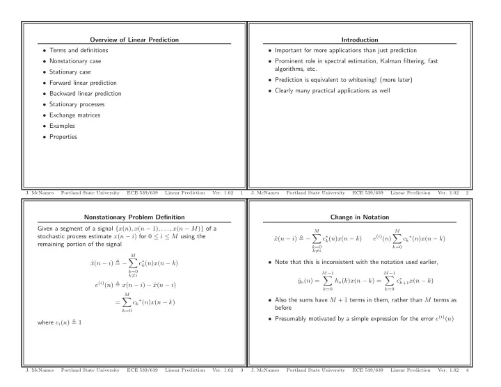
SLIDE 9

p = 1; % Number of steps ahead to predict M = 1:100; nM = length(M); NMSE = zeros(nM,1); for c0=1:nM, m = M(c0); % Filter length R = zeros(m,m); for c1=1:m, for c2=1:m, R(c1,c2) = rx(abs(c1-c2)+1); end; end; d = zeros(m,1); for c1=1:m, d(c1) = rx(c1+p); end; co = inv(R)*d; xh = filter(co,1,[zeros(p,1);x]); xh = xh(1:nx); NMSE(c0) = mean((x-xh).^2)/mean(x.^2); end; figure; FigureSet(1,’LTX’); h = plot(M,NMSE,’b’); set(h(1),’LineWidth’,0.8); AxisSet(8); xlabel(’M (samples)’); ylabel(’NMSE’); title(sprintf(’P:%d’,p)); xlim([0.5 M(end)+0.5]); ylim([0 1.05]); box off; print(’RESweepM’,’-depsc’);

J. McNames

Portland State University ECE 539/639 Linear Prediction

Ver. 1.02

35

FigureSet(1,’LTX’); AxisSet(8); print(’REAutocorrelation’,’-depsc’); %================================================ % Plot the Partial Autocorrelation %================================================ PartialAutocorrelation(x,fs,.5); FigureSet(1,’LTX’); AxisSet(8); print(’REPartialAutocorrelation’,’-depsc’); %================================================ % Plot the Power Spectral Density %================================================ BlackmanTukey(x,fs,10); FigureSet(1,’LTX’); AxisSet(8); print(’REBlackmanTukey’,’-depsc’); %================================================ % Plot the Spectrogram %================================================ NonparametricSpectrogram(decimate(x,5),fs/5,2); FigureSet(1,’LTX’); AxisSet(8); print(’RESpectrogram’,’-depsc’); %================================================ % Calculate the Auto- and Cross-Correlation %================================================ rx = Autocorrelation(x,fs,2); m = 25; % Filter length p = 1; % Number of steps ahead to predict R = zeros(m,m);

J. McNames

Portland State University ECE 539/639 Linear Prediction

Ver. 1.02

33

%================================================ % Sweep P for P=1 %================================================ P = 1:300; % Number of steps ahead to predict m = 25; nP = length(P); NMSE = zeros(nP,1); R = zeros(m,m); for c1=1:m, for c2=1:m, R(c1,c2) = rx(abs(c1-c2)+1); end; end; for c0=1:nP, p = P(c0); % Filter length d = zeros(m,1); for c1=1:m, d(c1) = rx(c1+p); end; co = inv(R)*d; xh = filter(co,1,[zeros(p,1);x]); xh = xh(1:nx); NMSE(c0) = mean((x-xh).^2)/mean(x.^2); end; figure; FigureSet(1,’LTX’); h = plot(P/fs,NMSE,’b’); set(h,’LineWidth’,0.8); set(h,’Marker’,’.’); set(h,’MarkerSize’,5); hold on; hb = plot([0 P(end)/fs],[1 1],’r:’); hold off;

J. McNames

Portland State University ECE 539/639 Linear Prediction

Ver. 1.02

36

for c1=1:m, for c2=1:m, R(c1,c2) = rx(abs(c1-c2)+1); end; end; d = zeros(m,1); for c1=1:m, d(c1) = rx(c1+p); end; co = inv(R)*d; xh = filter(co,1,[zeros(p,1);x]); xh = xh(1:nx); NMSE = mean((x-xh).^2)/mean(x.^2); %================================================ % Plot Segment of Signal and Predicted %================================================ figure; FigureSet(1,’LTX’); h = plot(t,x,’r’,t,xh,’g’); set(h(1),’LineWidth’,0.8); set(h(2),’LineWidth’,1.2); AxisSet(8); xlabel(’Time (s)’); ylabel(’Acceleration (scaled)’); title(sprintf(’NMSE:%5.3f P:%d M:%d’,NMSE,p,m)); legend(h,’Signal’,’Predicted’); xlim([t(1) 0.5]); ylim(prctile(x,[0.5 99.5])); box off; print(’RESignalPredicted’,’-depsc’); %================================================ % Sweep M for P=1 %================================================

J. McNames

Portland State University ECE 539/639 Linear Prediction

Ver. 1.02

34

SLIDE 10

AxisSet(8); xlabel(’P (s)’); ylabel(’NMSE’); title(sprintf(’M:%d’,m)); xlim([0 P(end)/fs]); ylim([0 1.05]); box off; print(’RESweepP’,’-depsc’);

J. McNames

Portland State University ECE 539/639 Linear Prediction

Ver. 1.02