
SLIDE 1
Outline Static Analysis: Symbolic Execution and Inductive - - PowerPoint PPT Presentation
Outline Static Analysis: Symbolic Execution and Inductive Verification Methods Overview TDDC90: Software Security Symbolic Execution Ahmed Rezine Hoare Triples and Deductive Reasoning IDA, Linkpings Universitet Hsttermin 2014 Static
■ syntactic analysis: scalable but neither sound nor complete ■ abstract interpretation sound but not complete
■ symbolic executions: complete but not sound ■ inductive methods: may require heavy human interaction in
1
2
3
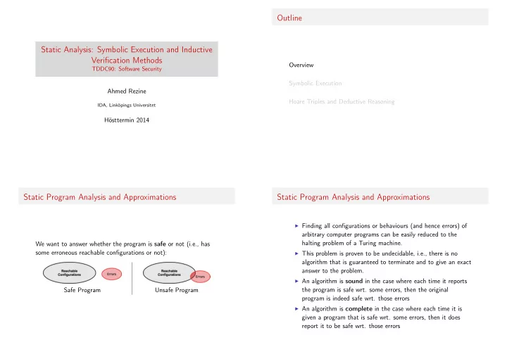
4
5
6
7
8
9
10
11
12
13
14
■ They can follow a concrete execution while collecting
■ They can treat some of the variables concretely, and some
■ if the pre-condition (-100 <= x && x <= 100) holds ■ then the implementation terminates, ■ after termination, the following post-condition holds
1
2
3
4
5
6
7
8
■ a predicate pre-condition P ■ an instruction stmt, ■ a predicate post-condition R
■ ❢true❣ x = y ❢(x == y)❣ ■ ❢(x == 1)&&(y == 2)❣ x = y ❢(x == 2)❣ ■ ❢(x ❃= 1)❣ y = 2 ❢(x == 0)❥❥(y ❁= 10)❣ ■ ❢(x ❃= 1)❣ (if(y == 2) then x = 0) ❢(x ❃= 0)❣ ■ ❢false❣ x = 1 ❢(x == 2)❣
■ wp(x = 3❀ x == 5) = (x == 5)[x❂3] = (3 == 5) = false ■ wp(x = 3❀ x ❃= 0) = (x ❃= 0)[x❂3] = (3 ❃= 0) = true ■ wp(x = y + 5❀ x ❃= 0) = (x ❃= 0)[x❂y + 5] = (y + 5 ❃= 0) ■ wp(x = 5 ✄ y + 2 ✄ z❀ x + y ❃= 0) = (x + y ❃=
■ P ✮ Inv ■ ❢Inv&&B❣ stmt ❢Inv❣ ■ (Inv&&!B)✮R
■ (i == j == 0) ✮ Inv ■ ❢Inv&&(i ❁ 10)❣ i = i + 1; j = j + 1 ❢Inv❣ ■ (Inv&&i ❃= 10)✮j == 10
■ P ✮ Inv ■ ❢Inv&&B❣ stmt ❢Inv❣ ■ (Inv&&!B)✮R
■ (Inv&&B) ✮ (v ❃ 0) ■ ❢Inv&&B&&v = v0❣ stmt ❢v ❁ v0❣