Outline Data cleaning and standardisation Febrl A parallel open - - PowerPoint PPT Presentation

Febrl – A parallel open source data linkage and geocoding system

Peter Christen, Tim Churches and others Data Mining Group, Australian National University Centre for Epidemiology and Research, New South Wales Department of Health Contacts: peter.christen@anu.edu.au tchur@doh.health.nsw.gov.au Project web page: http://datamining.anu.edu.au/linkage.html

Funded by the ANU, the NSW Department of Health, the Australian Research Council (ARC), and the Australian Partnership for Advanced Computing (APAC)

Peter Christen, May 2004 – p.1/32

Outline

Data cleaning and standardisation Data linkage and data integration Febrl overview Probabilistic data cleaning and standardisation Blocking / indexing Record pair classification Parallelisation in Febrl Data set generation Geocoding Outlook

Peter Christen, May 2004 – p.2/32

Data cleaning and standardisation (1)

Real world data is often dirty

Missing values, inconsistencies Typographical and other errors Different coding schemes / formats Out-of-date data

Names and addresses are especially prone to data entry errors Cleaned and standardised data is needed for

Loading into databases and data warehouses Data mining and other data analysis studies Data linkage and data integration

Peter Christen, May 2004 – p.3/32

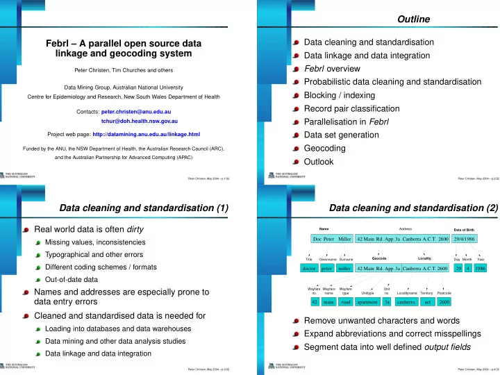
Data cleaning and standardisation (2)

42 Main 3a 2600 2600 3a App. Rd. Miller 3a 29/4/1986 42 Main Peter

• Rd. App.

1986 29 4

Address Name Geocode Locality

Doc 2600 A.C.T. Canberra Canberra A.C.T.

Title Givenname Surname Year Month Day Postcode Territory Localityname no. Unit Unittype

42

type Wayfare Wayfare name no. Wayfare

peter miller main canberra act apartment road doctor

Date of Birth

Remove unwanted characters and words Expand abbreviations and correct misspellings Segment data into well defined output fields

Peter Christen, May 2004 – p.4/32

Data linkage and data integration

The task of linking together records representing the same entity from one or more data sources If no unique identifier is available, probabilistic linkage techniques have to be applied Applications of data linkage

Remove duplicates in a data set (internal linkage) Merge new records into a larger master data set Create customer or patient oriented statistics Compile data for longitudinal studies

Data cleaning and standardisation are important first steps for successful data linkage

Peter Christen, May 2004 – p.5/32

Data linkage techniques

Deterministic or exact linkage

A unique identifier is needed, which is of high quality (precise, robust, stable over time, highly available) For example Medicare number (?)

Probabilistic linkage (Fellegi & Sunter, 1969)

Apply linkage using available (personal) information Examples: names, addresses, dates of birth

Other techniques

(rule-based, fuzzy approach, information retrieval)

Peter Christen, May 2004 – p.6/32

Febrl – Freely extensible biomedical record linkage

An experimental platform for new and improved linkage algorithms Modules for data cleaning and standardisation, data linkage, deduplication and geocoding Open source

https://sourceforge.net/projects/febrl/

Implemented in Python

http://www.python.org

Easy and rapid prototype software development Object-oriented and cross-platform (Unix, Win, Mac) Can handle large data sets stable and efficiently Many external modules, easy to extend

Peter Christen, May 2004 – p.7/32

Probabilistic data cleaning and standardisation

Three step approach

• 1. Cleaning

– Based on look-up tables and correction lists – Remove unwanted characters and words – Correct various misspellings and abbreviations

• 2. Tagging

– Split input into a list of words, numbers and separators – Assign one or more tags to each element of this list (using look-up tables and some hard-coded rules)

• 3. Segmenting

– Use either rules or a hidden Markov model (HMM) to assign list elements to output fields

Peter Christen, May 2004 – p.8/32

Cleaning

Assume the input component is one string

(either name or address – dates are processed differently)

Convert all letters into lower case Use correction lists which contain pairs of

• riginal:replacement strings

An empty replacement string results in removing the original string Correction lists are stored in text files and can be modified by the user Different correction lists for names and addresses

Peter Christen, May 2004 – p.9/32

Tagging

Cleaned strings are split at whitespace boundaries into lists of words, numbers, characters, etc. Using look-up tables and some hard-coded rules, each element is tagged with one or more tags Example:

Uncleaned input string: “Doc. peter Paul MILLER” Cleaned string: “dr peter paul miller” Word and tag lists:

[‘dr’, ‘peter’, ‘paul’, ‘miller’] [‘TI’, ‘GM/SN’, ‘GM’, ‘SN’ ]

Peter Christen, May 2004 – p.10/32

Segmenting

Using the tag list, assign elements in the word list to the appropriate output fields Rules based approach (e.g. AutoStan)

Example: “if an element has tag ‘TI’ then assign the corresponding word to the ‘Title’ output field” Hard to develop and maintain rules Different sets of rules needed for different data sets

Hidden Markov model (HMM) approach

A machine learning technique (supervised learning) Training data is needed to build HMMs

Peter Christen, May 2004 – p.11/32

Hidden Markov model (HMM)

Middlename End Surname Start Title Givenname

15% 85% 5% 65% 10% 5% 5% 25% 100% 20% 5% 75% 30% 55%

A HMM is a probabilistic finite state machine

Made of a set of states and transition probabilities between these states In each state an observation symbol is emitted with a certain probability distribution In our approach, the observation symbols are tags and the states correspond to the output fields

Peter Christen, May 2004 – p.12/32

HMM probability matrices

Middlename End Surname Start Title Givenname

15% 85% 5% 65% 10% 5% 5% 25% 100% 20% 5% 75% 30% 55%

State Observation Start Title Givenname Middlename Surname End TI – 96% 1% 1% 1% – GM – 1% 35% 33% 15% – GF – 1% 35% 27% 14% – SN – 1% 9% 14% 45% – UN – 1% 20% 25% 25% –

Peter Christen, May 2004 – p.13/32

HMM data segmentation

Middlename End Surname Start Title Givenname

15% 85% 5% 65% 10% 5% 5% 25% 100% 20% 5% 75% 30% 55%

For an observation sequence we are interested in the most likely path through a given HMM

(in our case an observation sequence is a tag list)

The Viterbi algorithm is used for this task

(a dynamic programming approach)

Smoothing is applied to account for unseen data

(assign small probabilities for unseen observation symbols)

Peter Christen, May 2004 – p.14/32

HMM segmentation example

Middlename End Surname Start Title Givenname

15% 85% 5% 65% 10% 5% 5% 25% 100% 20% 5% 75% 30% 55%

Input word and tag list

[‘dr’, ‘peter’, ‘paul’, ‘miller’] [‘TI’, ‘GM/SN’, ‘GM’, ‘SN’ ]

Two example paths through the HMM

1: Start -> Title (TI) -> Givenname (GM) -> Middlename (GM) -> Surname (SN) -> End 2: Start -> Title (TI) -> Surname (SN) -> Givenname (GM) -> Surname (SN) -> End

Peter Christen, May 2004 – p.15/32

HMM training (1)

Both transition and observation probabilities need to be trained using training data

(maximum likelihood estimates (MLE) are derived by accumulating frequency counts for transitions and

• bservations)

Training data consists of records, each being a sequence of tag:hmm_state pairs Example (2 training records):

# ‘42 / 131 miller place manly 2095 new_south_wales’ NU:unnu,SL:sla,NU:wfnu,UN:wfna1,WT:wfty,LN:loc1,PC:pc,TR:ter1 # ‘2 richard street lewisham 2049 new_south_wales’ NU:wfnu,UN:wfna1,WT:wfty,LN:loc1,PC:pc,TR:ter1

Peter Christen, May 2004 – p.16/32

HMM training (2)

A bootstrapping approach is applied for semi- automatic training

• 1. Manually edit a small number of training records and

train a first rough HMM

• 2. Use this first HMM to segment and tag a larger number
• f training records
• 3. Manually check a second set of training records, then

train an improved HMM

Only a few person days are needed to get a HMM that results in an accurate standardisation

(instead of weeks or even months to develop rules)

Peter Christen, May 2004 – p.17/32

Address standardisation results

Various NSW Health data sets

HMM1 trained on 1,450 Death Certificate records HMM2 contains HMM1 plus 1,000 Midwifes Data Collection training records HMM3 is HMM2 plus 60 unusual training records

AutoStan rules (for ISC) developed over years

HMM/Method Test Data Set HMM HMM HMM Auto (1,000 records each) 1 2 3 Stan Death Certificates 95.7% 96.8% 97.6% 91.5% Inpatient Statistics Collection 95.7% 95.9% 97.4% 95.3%

Peter Christen, May 2004 – p.18/32

Name standardisation results

NSW Midwifes Data Collection (1990 - 2000)

(around 963,000 records, no medical information)

10-fold cross-validation study with 10,000 random records (9,000 training and 1,000 test records) Both Febrl rule based and HMM data cleaning and standardisation

Rules were better because most names were simple (not much structure to learn for HMM)

Min Max Average StdDev HMM 83.1% 97.0% 92.0%

• 4.7%

Rules 97.1% 99.7% 98.2%

• 0.7%

Peter Christen, May 2004 – p.19/32

Blocking / indexing

Number of possible links equals the product of the sizes of the two data sets to be linked Performance bottleneck in a data linkage system is usually the (expensive) evaluation of similarity measures between record pairs Blocking / indexing techniques are used to reduce the large amount of record comparisons Febrl contains (currently) three indexing methods

Standard blocking Sorted neighbourhood approach Fuzzy blocking using

• grams (e.g. bigrams)

Peter Christen, May 2004 – p.20/32

Record pair classification

For each record pair compared a vector containing matching weights is calculated

Example:

Record A: [’dr’, ’peter’, ’paul’, ’miller’] Record B: [’mr’, ’pete’, ’’, ’miller’] Matching weights: [0.2, 0.8, 0.0, 2.4]

Matching weights are used to classify record pairs as links, non-links, or possible links Fellegi & Sunter classifier simply sums all the weights, then uses two thresholds to classify Improved classifiers are possible

(for example using machine learning techniques)

Peter Christen, May 2004 – p.21/32

Final linkage decision

The final weight is the sum of weights of all fields

Record pairs with a weight above an upper threshold are designated as a link Record pairs with a weight below a lower threshold are designated as a non-link Record pairs with a weight between are possible link

−5 5 10 15 20 Lower threshold Upper threshold Total matching weight lower weight Many more with Peter Christen, May 2004 – p.22/32

Parallelisation

Implemented transparently to the user Currently using MPI via Python module PyPar Use of supercomputing centres is problematic (privacy)

Alternative: In-house office clusters Some initial performance results (on Sun SMP)

1 1.5 2 2.5 3 1 2 3 4 Speedup

Number of processors Step 1 - Loading and indexing 20,000 records 100,000 records 200,000 records 1 1.5 2 2.5 3 3.5 4 1 2 3 4 Speedup

Number of processors Step 2 - Record pair comparison and classification 20,000 records 100,000 records 200,000 records

Peter Christen, May 2004 – p.23/32

Data set generation

Difficult to acquire data for testing and evaluation

(as data linkage deals with names and addresses)

Also, linkage status is often not known

(hard to evaluate and test new algorithms)

Febrl contains a data set generator

Uses frequency tables for given- and surnames, street names and types, suburbs, postcodes, etc. Duplicate records are created via random introduction of modifications (like insert/delete/transpose characters, swap field values, delete values, etc.)

Peter Christen, May 2004 – p.24/32

Data set generation – Example

Data set with 4 original and 6 duplicate records

REC_ID, ADDRESS1, ADDRESS2, SUBURB rec-0-org, wylly place, pine ret vill, taree rec-0-dup-0, wyllyplace, pine ret vill, taree rec-0-dup-1, pine ret vill, wylly place, taree rec-0-dup-2, wylly place, pine ret vill, tared rec-0-dup-3, wylly parade, pine ret vill, taree rec-1-org, stuart street, hartford, menton rec-2-org, griffiths street, myross, kilda rec-2-dup-0, griffith sstreet, myross, kilda rec-2-dup-1, griffith street, mycross, kilda rec-3-org, ellenborough place, kalkite homestead, sydney

Each record is given a unique identifier, which allows the evaluation of accuracy and error rates for data linkage

Peter Christen, May 2004 – p.25/32

Geocoding

The process of matching addresses with geographic locations (longitude and latitude) Geocoding tasks

Preprocess the geocoded reference data (cleaning, standardisation and indexing) Clean and standardise the user addresses (Fuzzy) match of user addresses with the reference data Return location and match status

Match status: address, street or locality level Geocode reference data used: G-NAF

Peter Christen, May 2004 – p.26/32

Geocoded national address file

G-NAF: Available since early 2004

(PSMA, http://www.g-naf.com.au/)

Source data from 13 organisations

(around 32 million source records)

Preprocessed into 22 normalised database tables

Adress Site Geocode Adress Site Adress Detail Adress Alias Locality Locality Alias Street Street Locality Geocode Street Locality Alias Geocode Locality

1 1 1 n n n n 1 1 n 1 n 1 n 1 1 1 n 1 n 1 n Peter Christen, May 2004 – p.27/32

Febrl geocoding system

G−NAF data files Febrl clean and standardise indexes Build inverted data files Inverted index Febrl geocode match engine Febrl clean and standardise file User data Geocoded user data file

Geocoding module Process−GNAF module

input data Web interface Geocoded Web data GIS data AustPost data

Web server module

Only NSW G-NAF data available

(around 4 million address, 58,000 street and 5,000 locality records)

Additional Australia Post and GIS data used

(for data imputing and to calculate neighbouring regions)

Peter Christen, May 2004 – p.28/32

Processing G-NAF files

Clean and standardise Build inverted indexes

LOCALITY_PID, LOCALITY_NAME, STATE_ABBREV, POSTCODE 60310919, sydney, nsw, 2000 60709845, north_sydney, nsw, 2059 60309156, north_sydney, nsw, 2060 61560124, the_rocks, , 2000

• - - - - - - - - - - - - - - - - - - - - - - - - - - - - -

locality_name_index = [’north_sydney’:(60709845,60309156), ’sydney’:(60310919), ’the_rocks’:(61560124)] state_abbrev_index = [’nsw’:(60310919,60709845,60309156)] postcode_index = [’2000’:(60310919,61560124), ’2059’:(60709845), ’2060’:(60309156)]

Peter Christen, May 2004 – p.29/32

Febrl geocoding match engine

Uses cleaned and standardised user address(es) and G-NAF inverted index data Fuzzy rule based approach

• 1. Find street match set (street name, type and number)
• 2. Find postcode and locality match set (with no, then

direct, then indirect neighbour levels)

• 3. Intersect postcode and locality sets with street match set

(if no match increase neighbour level and go back to 2.)

• 4. Refine with unit, property, and building match sets
• 5. Retrieve corresponding locality (or localities)
• 6. Return locality and match status (address, street or

locality level match; none, one or many matches)

Peter Christen, May 2004 – p.30/32

Outlook

Several research areas

Improving probabilistic data standardisation New and improved blocking / indexing methods Apply machine learning techniques for record pair classification Improve performances (scalability and parallelism)

Project web page

http://datamining.anu.edu.au/linkage.html

Febrl is an ideal experimental platform to develop, implement and evaluate new data standardisation and data linkage algorithms and techniques

Peter Christen, May 2004 – p.31/32

Contributions / Acknowledgments

Dr Markus Hegland (ANU Mathematical Sciences Institute) Dr Lee Taylor (New South Wales Health Department, Centre for Epidemiology and Research) Ms Kim Lim (New South Wales Health Department, Centre for Epidemiology and Research) Mr Alan Willmore (New South Wales Health Department, Centre for Epidemiology and Research) Mr Karl Goiser (ANU Computer Science PhD student) Mr Justin Zhu (ANU Computer Science honours student, 2002) Mr David Horgan (ANU Computer Science summer student, 2003/2004) Mr Puthick Hok (ANU Computer Science honours student, 2004)

Peter Christen, May 2004 – p.32/32