Outline 1 - - PDF document

SLIDE 1

• † ‡

† ‡JST

2015 12 24

• 1 / 95

Outline

1

• 2
• 3
• n ≫ p

n ≪ p

• 4
• 5
• 2 / 95
• d = 10000 n = 1000
• ()

3 / 95

:

1992 Donoho and Johnstone Wavelet shrinkage (Soft-thresholding) 1996 Tibshirani Lasso 2000 Knight and Fu Lasso (n ≫ p) 2006 Candes and Tao,

• Donoho

(p ≫ n) 2009 Bickel et al., Zhang

• (Lasso , p ≫ n)

2013 van de Geer et al.,

• Lockhart et al.

(p ≫ n)

L1 (2010) .

4 / 95

Outline

1

• 2
• 3
• n ≫ p

n ≪ p

• 4
• 5
• 5 / 95
• ≪
• 6 / 95

SLIDE 2

• ≪

≫

• 6 / 95
• ≪
• Lasso
• R. Tsibshirani (1996). Regression shrinkage and selection via the lasso.
• J. Royal. Statist. Soc B., Vol. 58, No. 1, pages 267–288.

14728 (2015 12 23 )

7 / 95

• X = (Xij) ∈ Rn×p,

Y = (Yi) ∈ Rn p () ≫ n (). β∗ ∈ Rp: d (). : Y = Xβ∗ + ǫ (Yi = p

j=1 Xijβ∗ j + ǫi)

(i = 1, . . . , n)) (Y , X) β∗ d

• 8 / 95
• X = (Xij) ∈ Rn×p,

Y = (Yi) ∈ Rn p () ≫ n (). β∗ ∈ Rp: d (). : Y = Xβ∗ + ǫ (Yi = p

j=1 Xijβ∗ j + ǫi)

(i = 1, . . . , n)) (Y , X) β∗ d

Mallows’ Cp, AIC:

ˆ βMC = argmin

β∈Rp

Y − Xβ2 + 2σ2β0 β0 = |{j | βj = 0}|. 2p NP-

8 / 95

http://www.astroml.org/sklearn_tutorial/practical.html

y = b + β1x + β2x2 + · · · + βdxd + ǫ

9 / 95

Lasso

Mallows’ Cp : ˆ βMC = argmin

β∈Rp

Y − Xβ2 + 2σ2β0. : β0

Lasso [L1 ]

ˆ βLasso = argmin

β∈Rp

Y − Xβ2 + λβ1

β1 = p

j=1 |βj|.

L1 L0 [−1, 1]p () L1 Lov´ asz

10 / 95

SLIDE 3

Lasso

p = n, X = I ˆ βLasso = argmin

β∈Rp

1 2Y − β2 + Cβ1 ⇒ ˆ βLasso,i = argmin

b∈R

1 2(yi − b)2 + C|b| =

• sign(yi)(yi − C)

(|yi| > C) (|yi| ≤ C).

11 / 95

Lasso

ˆ β = arg min

β∈Rp

1 nXβ − Y 2

2 + λn p

• j=1

|βj|.

12 / 95

• ˆ

β = arg min

β∈Rp

1 nXβ − Y 2

2 + λn p

• j=1

|βj|.

Theorem (Lasso )

C ˆ β − β∗2

2 ≤ C dlog(p)

n . log(p) d

• 13 / 95
• Y = Xβ + ǫ.

n = 1, 000, p = 10, 000, d = 500.

1000 2000 3000 4000 5000 6000 7000 8000 9000 10000 1 2 3 4 5 6 7 8 9 10

True

14 / 95

• Y = Xβ + ǫ.

n = 1, 000, p = 10, 000, d = 500.

1000 2000 3000 4000 5000 6000 7000 8000 9000 10000

• 2

2 4 6 8 10 12

True Lasso

14 / 95

• Y = Xβ + ǫ.

n = 1, 000, p = 10, 000, d = 500.

1000 2000 3000 4000 5000 6000 7000 8000 9000 10000

• 2

2 4 6 8 10 12

True Lasso LeastSquares

14 / 95

SLIDE 4

Outline

1

• 2
• 3
• n ≫ p

n ≪ p

• 4
• 5
• 15 / 95

Lasso

Lasso: min

β∈Rp

1 n

n

• i=1

(yi − x⊤

i β)2 + β1

• .
• 16 / 95

Lasso

Lasso: min

β∈Rp

1 n

n

• i=1

(yi − x⊤

i β)2 + β1

• .

: min

w∈Rp

1 n

n

• i=1

ℓ(zi, β) + ψ(β). L1

16 / 95

L1

17 / 95

• C
• g∈G

βg

• 18 / 95
• Lounici et al. (2009)

T : y (t)

i

≈ x(t)⊤

i

β(t) (i = 1, . . . , n(t), t = 1, . . . , T). min

β(t) T

• t=1

n(t)

• i=1

(yi − x(t)⊤

i

β(t))2 + C

p

• k=1

(β(1)

k , . . . , β(T) k

)

• .

β(1)β(2) β(T)

• 19 / 95

SLIDE 5

• Lounici et al. (2009)

T : y (t)

i

≈ x(t)⊤

i

β(t) (i = 1, . . . , n(t), t = 1, . . . , T). min

β(t) T

• t=1

n(t)

• i=1

(yi − x(t)⊤

i

β(t))2 + C

p

• k=1

(β(1)

k , . . . , β(T) k

)

• .

β(1)β(2) β(T)

• 19 / 95
• W : M × N

W Tr = Tr[(WW ⊤)

1 2 ] =

min{M,N}

• j=1

σj(W )

σj(W ) W j () = L1 =

20 / 95

:

• A

B C · · · X 1 4 8 * · · · 2 2 2 * 2 · · · * 3 2 4 * · · · * . . . (e.g., Srebro et al. (2005), NetFlix Bennett and Lanning (2007))

21 / 95

:

1 A B C · · · X 1 4 8 4 · · · 2 2 2 4 2 · · · 1 3 2 4 2 · · · 1 . . . (e.g., Srebro et al. (2005), NetFlix Bennett and Lanning (2007))

• (i,j)∈T

(Yi,j − Wi,j)2 + λW Tr

21 / 95

:

W*=

N M 映画 ユーザ

: Rademacher Complexity: Srebro et al. (2005). Compressed sensing: Cand` es and Tao (2009), Cand` es and Recht (2009).

22 / 95

:

(Anderson, 1951, Burket, 1964, Izenman, 1975) (Argyriou et al., 2008)

• =

W* n Y X N M N W

+

W ∗ .

23 / 95

SLIDE 6

• xk ∼ N(0, Σ) (i.i.d., Σ ∈ Rp×p),
• Σ = 1

n

n

k=1 xkx⊤ k .

ˆ S = argmin

S:

• − log(det(S)) + Tr[S

Σ] + λ

p

• i,j=1

|Si,j|

• .

(Meinshausen and B uhlmann, 2006, Yuan and Lin, 2007, Banerjee et al., 2008)

Σ S Si,j = 0 ⇔ X(i), X(j)

• 24 / 95

NASDAQ 50 . (2011 1 4 2014 12 31 ) (Lie Michael, Bachelor thesis)

25 / 95

() Fused Lasso

ψ(β) = C

• (i,j)∈E

|βi − βj|.

(Tibshirani et al. (2005), Jacob et al. (2009)) Fused lasso (Tibshirani and Taylor ‘11) TV (Chambolle ‘04)

26 / 95

• SCAD (Smoothly Clipped Absolute Deviation) (Fan and Li, 2001)

MCP (Minimax Concave Penalty) (Zhang, 2010) Lq (q < 1), Bridge (Frank and Friedman, 1993)

• 27 / 95

L1

Adaptive Lasso (Zou, 2006) ˜ β ψ(β) = C

p

• j=1

|βj| |˜ βj|γ

Lasso ()

• (Hastie and Tibshirani, 1999, Ravikumar et al., 2009)

f (x) = p

j=1 fj(xj)

fj ∈ Hj (Hj: ) ψ(f ) = C

p

• j=1

fjHj

Group Lasso Multiple Kernel Learning

28 / 95

Outline

1

• 2
• 3
• n ≫ p

n ≪ p

• 4
• 5
• 29 / 95

SLIDE 7

• Y = Xβ∗ + ǫ.

Y ∈ Rn : , X ∈ Rn×p : , ǫ = [ǫ1, . . . , ǫn]⊤ ∈ Rn.

• 30 / 95

n ≫ p

31 / 95

Lasso

p n → ∞

1 nX ⊤X p

− → C ≻ O. ǫi 0 σ2 .

Theorem (Lasso (Knight and Fu, 2000))

λn √n → λ0 ≥ 0 √n(ˆ β − β∗)

d

− → argmin

u

V (u), V (u) = u⊤Cu − 2u⊤W + λ0 p

j=1[ujsign(β∗ j )1(β∗ j = 0) + |uj|1(β∗ j = 0)],

W ∼ N(0, σ2C). ˆ β √n-consistent β∗

j = 0 ˆ

βj 0

• ˆ

β = argminβ

1 nY − Xβ2 + λn

p

j=1 |βj|.

32 / 95

Adaptive Lasso

˜ β ˆ β = argmin

β

1 nY − Xβ2 + λn

p

• j=1

|βj| |˜ βj|γ .

Theorem (Adaptive Lasso (Zou, 2006))

λn √n → 0, λnn

1+γ 2

→ ∞

1

limn→∞ P(ˆ J = J) → 1 (ˆ J := {j | |ˆ βj| = 0}, J := {j | |β∗

j | = 0}),

2

√n(ˆ βJ − β∗

J ) d

− → N(0, σ2C −1

JJ ).

• β∗ (β∗

j = O(1/√n)

)

33 / 95

n ≪ p

34 / 95

Lass

ˆ β = arg min

β∈Rp

1 nXβ − Y 2

2 + λn p

• j=1

|βj|.

Theorem (Lasso

(Bickel et al., 2009, Zhang, 2009)) Restricted eigenvalue condition (Bickel et al., 2009)

maxi,j |Xij| ≤ 1 E[eτξi] ≤ eσ2τ 2/2 (∀τ > 0) , 1 − δ ˆ β − β∗2

2 ≤ C d log(p/δ)

n . log(p) d

• 35 / 95

SLIDE 8

Lasso minimax

Theorem ( (Raskutti and Wainwright, 2011))

1/2 min

ˆ β:

max

β∗:d- ˆ

β − β∗2 ≥ C d log(p/d) n . Lasso minimax ( d log(d)

n

) Multiple Kernel Learning : Raskutti et al. (2012), Suzuki and Sugiyama (2013).

36 / 95

(Restricted eigenvalue condition)

A = 1

nX ⊤X

Definition ( (RE(k′, C))) φRE(k′, C) = φRE(k′, C, A) := inf

J⊆{1,...,n},v∈Rp: |J|≤k′,CvJ1≥vJc 1

v ⊤Av vJ2

2

φRE > 0

• J
• 37 / 95

(Compatibility condition)

A = 1

nX ⊤X

Definition ( (COM(J, C)))

φCOM(J, C) = φCOM(J, C, A) := inf

v∈Rp: CvJ1≥vJc 1

k v ⊤Av vJ2

1

φCOM > 0 |J| ≤ k′ RE

38 / 95

(Restricted isometory condition)

Definition ( (RI(k′, δ)) (Candes and Tao, 2005))

1 > δ > 0 (1 − δ)β2 ≤ Xβ2 ≤ (1 + δ)β2 k′- β ∈ Rp Johnson-Lindenstrauss .

• 39 / 95
• ˆ

β : Lasso . J := {j | β∗

j = 0}. d := |J|.

• 1

nX(ˆ

β − β∗)2

2

ˆ β − β∗2

2

ˆ β − β∗2

1

RI(Cd, δ)

• +

⇓ RE(2d, 3)

• d log(p)

n d log(p) n d2 log(p) n ⇓ COM(J, 3)

• d log(p)

n d2 log(p) n d2 log(p) n

• B¨

uhlmann and van de Geer (2011) (Candes and Tao, 2005) (Cand` es, 2008). RI RE Rudelson and Zhou (2013)

40 / 95

(RE)

• p Z : E[Z, z2] = z2

2 (∀z ∈ Rp).

Zψ2 : Zψ2 = supz∈Rp,z=1 inft{t | E[exp(Z, z)2/t2] ≤ 2}.

• 1. Z = [Z1, Z2, . . . , Zn]⊤ ∈ Rn×p Zi ∈ Rp
• 2. Σ ∈ Rp×p X = ZΣ

Theorem (Rudelson and Zhou (2013))

Ziψ2 ≤ κ (∀i) c0 m = c0

maxi(Σi,i)2 φ2

RE(k,9,Σ)

n ≥ 4c0mκ4 log(60ep/(mκ)) P

• φRE(k, 3,

Σ) ≥ 1 2φRE(k, 9, Σ)

• ≥ 1 − 2 exp(−n/(4c0κ4)).
• ⇒

41 / 95

SLIDE 9

• : Massart (2003), Bunea et al. (2007), Rigollet and

Tsybakov (2011). min

β∈Rp Y − Xβ2 + Cσ2β0

• 1 + log
• p

β0

• .

Bayes : Dalalyan and Tsybakov (2008), Alquier and Lounici (2011), Suzuki (2012). : X : 1 nXβ∗ − X ˆ β2 ≤ Cσ2 d n log

• 1 + p

d

• .
• 42 / 95
• 43 / 95
• ()

yi =

p

• j=1

x(j)

i

bj + ǫi − → yi =

p

• j=1

fj(x(j)

i

) + ǫi

44 / 95

• ()

yi =

p

• j=1

x(j)

i

bj + ǫi − → yi =

p

• j=1

fj(x(j)

i

) + ǫi

44 / 95

Multiple Kernel Learning

Multiple Kernel Learning (MKL) (Lanckriet et al., 2004, Bach et al., 2004) ˆ f =

M

• m=1

ˆ fm ← min

fm∈Hm n

• i=1
• yi −

M

• m=1

fm(xi) 2 + C

M

• m=1

fmHm (Hm: )

• : ˆ

fm 0. () (Sonnenburg et al., 2006, Rakotomamonjy et al., 2008, Suzuki and Tomioka, 2009)

• 45 / 95

Multiple Kernel Learning

Multiple Kernel Learning (MKL) (Lanckriet et al., 2004, Bach et al., 2004) ˆ f =

M

• m=1

ˆ fm ← min

fm∈Hm n

• i=1
• yi −

M

• m=1

fm(xi) 2 + C

M

• m=1

fmHm (Hm: )

• : ˆ

fm 0. () (Sonnenburg et al., 2006, Rakotomamonjy et al., 2008, Suzuki and Tomioka, 2009)

• M

m=1 fmHm

− → ψ((fmHm)M

m=1),

e.g., ℓp- (Micchelli and Pontil, 2005, Kloft et al., 2009)

• (Shawe-Taylor, 2008, Tomioka and Suzuki, 2009)Variable Sparsity Kernel

Learning (VSKL) (Aflalo et al., 2011).

45 / 95

SLIDE 10

• (Gehler&Nowozin, CVPR2009)
• (Widmer et al., BMC Bioinformatics 2010)

Time varying coefficient model

f(t)(x) = β⊤

(t)x (Lu et al., 2015)

46 / 95

• .

1

(Suzuki, 2011) ˆ f − f ∗2

L2(Π) = Op

• M1− 2s

1+s n− 1 1+s (1ψ∗f ∗ψ) 2s 1+s + M log(M)

n

• .

2

elastic-net (Suzuki and Sugiyama, 2013)

(L1) ˆ f − f ∗2

L2(Π) = Op

• d

1−s 1+s n− 1 1+s R 2s 1+s

1,f ∗ + d log(M)

n

• ,

(Elastic) ˆ f − f ∗2

L2(Π) = Op

• d

1+q 1+q+s n− 1+q 1+q+s R 2s 1+q+s

2,g∗

+ d log(M) n

• ,

3

: + (Suzuki, 2012) EY1:n|x1:n

• ˆ

f − f o2

n

• = Op

 

m∈I0

n−

1 1+sm + |I0|

n log Me κ|I0|   . Restricted Eigenvalue Condition

• 47 / 95

(s)

0 < s < 1: . (cf., Mercer ): km(x, x′) = ∞

ℓ=1 µℓ,mφℓ,m(x)φℓ,m(x′),

{φℓ,m}∞

ℓ=1 L2(P) .

(s)

0 < s < 1 µℓ,m ≤ Cℓ− 1

s

(∀ℓ, m). s s . s : Op(n−

1 1+s ).

Proposition (Steinwart et al. (2009))

µℓ,m ∼ ℓ− 1

s ⇔ log N(B(Hm), ǫ, L2(P)) ∼ ǫ−2s 48 / 95

• 映画

ユーザ

Movie User Context

• −

→ () Xij = d

r=1 u(1) r,i u(2) r,j

Xijk = d

r=1 u(1) r,i u(2) r,j u(3) r,k

49 / 95

• 1

1 3 1 2 2 2 4 2 4 2 1 3 2 41 2 3 2 3 4 2 1 3 2 2 1 22 1 4 1 1 3 2 4 4 1 41 3 2 1 3 2

User Item Context Rating Prediction

• Task type 1

Task type 2 feature

()

• 50 / 95
• Yi = Xi, A∗ + Wi.

A∗, Xi ∈ RM1×...MK : . Xi, A∗ :=

j1,...,jK Xi,(j1,...,jK )A∗ j1,...,jK .

Wi ∼ N(0, σ2): observational noise. E.g., Xi = ej1 ⊗ ej2 ⊗ · · · ⊗ ejK . : A∗ “”.

• 51 / 95

SLIDE 11

• Yi = Xi, A∗ + Wi.

A∗, Xi ∈ RM1×...MK : . Xi, A∗ :=

j1,...,jK Xi,(j1,...,jK )A∗ j1,...,jK .

Wi ∼ N(0, σ2): observational noise. E.g., Xi = ej1 ⊗ ej2 ⊗ · · · ⊗ ejK . : A∗ “”. : min

A∈RM1×M2×···×MK n

• i=1

(Yi − Xi, A∗)2 + pen(A). CP- Schatten-1 (Tomioka et al., 2011) Schatten-1 (Tomioka and Suzuki, 2013)

51 / 95

: CP-

CP- (Canonical Polyadic Decomp.) (Hitchcock, 1927a,b)

(figure is from (Kolda and Bader, 2009))

Xijk = d

r=1 airbjrckr =: [[A, B, C]].

CP- CP-. CP- NP-. CP- (). NP-

52 / 95

Schatten-1

| | |A| | |S1/1 :=

K

• k=1

A(k)Tr

Schatten-1

• A = arg min

A

| | |Y − A| | |2

F + λn|

| |A| | |S1/1. Tucker-. − → A A(1) A(2) A(3)

53 / 95

Schatten-1

| | |A| | |S1/1 := inf

A=A1+A2+···+AK K

• k=1

A(k)

k Tr

Schatten1

• A = arg min

A

| | |Y − A| | |2

F + λn|

| |A| | |S1/1, s.t. A =

K

• k=1

Ak, A(k′)

k

S∞ ≤ α K

• N/nk′ (∀k′ = k).
• A

= A1 + A2 + A3 ↓ ↓ ↓ A(1)

1

A(2)

2

A(3)

3

54 / 95

• min

A∈RM1×M2×···×MK

1 n

n

• i=1

(Yi − Xi, A)2 + pen(A). ✓ ✏ (Tomioka et al., 2011)

1 N |

| | A − A∗| | |2

F ≤ C n

• 1

K

K

k=1(√Mk +

• N/Mk)

2

1 K

K

k=1

√rk 2

(Tomioka and Suzuki, 2013):

1 N |

| | A − A∗| | |2

F ≤ C n

• maxk(√Mk +
• N/Mk)

2 mink rk

Square deal (Mu et al., 2014):

1 M ˆ

A − A∗2

2 ≤ C min{

k∈I1 rk , k∈I2 rk }

n

• k∈I1 Mk +

k∈I2 Mk

• ,

I1 I2 {1, . . . , K} . ✒ ✑ : . : .

55 / 95

• .

56 / 95

SLIDE 12

• A∗max,2 ≤ Rσp .

()

Theorem

n, {Mk}k C

()

EY1:n|X1:n 1 2σ2

• A − A∗2

ndΠ(A|X1:n, Y1:n)

• ≤C d(K

k=1 Mk)

n

• 1 ∨ R2

log

• K

σK

p

ξ

√ nRK

• .

()

EY1:n|X1:n 1 2σ2

• A − A∗2

L2dΠ(A|X1:n, Y1:n)

• ≤C d(K

k=1 Mk)

n

• 1 ∨ R2(K+1)

log

• K

σK

p

ξ

√ nRK

• .

57 / 95

• Hd(R) :=
• A ∈ RM1×···×MK | CP- d, Amax,2 ≤ R
• .

( d )

Theorem

Hd(R) : min

• A

max

A∗∈Hd(R) E[

A − A∗2

L2] d(M1 + · · · + MK)

n . log

58 / 95

• Figure: ( Schatten-1 ) .

59 / 95

• Figure: : The scaled predictive accuracy (left) and the actual predictive

accuracy (right) against the number of samples.

scaled accuracy = actual accuracy d(K

k=1 Mk)/n

60 / 95

Outline

1

• 2
• 3
• n ≫ p

n ≪ p

• 4
• 5
• 61 / 95
• Lasso ˆ

β . (van de Geer et al., 2014, Javanmard and Montanari, 2014) ✓ ✏ ˜ β = ˆ β + MX ⊤(Y − X ˆ β) ✒ ✑ M (X ⊤X)−1 ˜ β = β∗ + (X ⊤X)−1X ⊤ǫ. () : p ≫ n X ⊤X

62 / 95

SLIDE 13

M : min

M∈Rp×p

| ΣM⊤ − I|∞.

(| · |∞ )

Theorem (Javanmard and Montanari (2014))

ǫi ∼ N(0, σ2) (i.i.d.) √n(˜ β − β∗) = Z + ∆, Z ∼ N(0, σ2M ΣM⊤), ∆ = √n(M Σ − I)(β∗ − ˆ β). X λn = cσ

• log(p)/n

∆∞ = Op

• d log(p)

√n

• .

n ≫ d2 log2(p) ∆ ≈ 0 √n(˜ β − β∗)

63 / 95

M : min

M∈Rp×p

| ΣM⊤ − I|∞.

(| · |∞ )

Theorem (Javanmard and Montanari (2014))

√n(˜ β − β∗) = Z

• +

∆

• X

n ≫ d2 log2(p) ∆ ≈ 0 √n(˜ β − β∗)

63 / 95

• (a) 95%.

(n, p, d) = (1000, 600, 10). (b) p CDF. (n, p, d) = (1000, 600, 10).

Javanmard and Montanari (2014)

64 / 95

(Lockhart et al., 2014)

500 1000 1500 2000 2500 3000 −600 −400 −200 200 400 600 L1 Norm Coefficients 2 4 6 8 10 10

• 65 / 95

(Lockhart et al., 2014)

500 1000 1500 2000 2500 3000 −600 −400 −200 200 400 600 L1 Norm Coefficients 2 4 6 8 10 10

J = supp(ˆ β(λk)), J∗ = supp(β∗), ˜ β(λk+1) := argmin

β:βJ∈R|J|,βJc =0

Y − XJβJ2 + λk+1βJ1. J∗ ⊆ J ( β∗

j = 0)

Tk =

• Y , X ˆ

β(λk+1) − Y , X ˜ β(λk+1)

• /σ2

d

− → Exp(1) (n, p → ∞).

65 / 95

Outline

1

• 2
• 3
• n ≫ p

n ≪ p

• 4
• 5
• 66 / 95

SLIDE 14

• R(β) =

n

• i=1

ℓ(yi, x⊤

i β)

• f (β):

+ ψ(β)

• = f (β) + ψ(β)

ψ f ψ R

• 67 / 95
• R(β) =

n

• i=1

ℓ(yi, x⊤

i β)

• f (β):

+ ψ(β)

• = f (β) + ψ(β)

ψ f ψ R

• L1 ψ(β) = C p

j=1 |βj| .

minb{(b − y)2 + C|b|} .

67 / 95

• 1 j ∈ {1, . . . , p}

2 j βj

• β(k+1)

j

← argminβj R([β(k)

1 , . . . , βj, . . . , β(k) p ]).

gj = ∂f (β(k))

∂βj

• β(k+1)

j

← argminβj gj, βj + ψj(βj) + ηk

2 βj − β(k) j

2. :

• 68 / 95
• failure

success

: , . f (x) = p

j=1 fj(xj).

69 / 95

• minx{P(x)} = minx{f (x) + ψ(x)} = minx{f (x) + p

j=1 ψj(xj)}.

: f γ- (|∂xjf (x) − ∂xjf (x + aej)| ≤ γa) (Saha and Tewari, 2013, Beck and Tetruashvili, 2013) P(x(t)) − R(x∗) ≤ γpx(0)−x∗2

2t

= O(pγ/t). (Nesterov, 2012, Richt´

arik and Tak´ aˇ c, 2014) : O(pγ/t). Nesterov : O(γ(p/t)2) (Fercoq and Richt´ arik, 2013). f α-: O(exp(−C(α/γ)t/p)). f α- + : O(exp(−C

• α/γt/p)) (Lin et al., 2014).
• : Wright (2015).

70 / 95

• Hydra: (Richt´

arik and Tak´ aˇ c, 2013, Fercoq et al., 2014). Lasso (p = 5 × 108, n = 109) Hydra (Richt´ arik and Tak´ aˇ c, 2013)128 4,096

71 / 95

SLIDE 15

• f (β)
• +ψ(β)

gk ∈ ∂f (β(k)), ¯ gk = 1

k

k

τ=1 gτ.

: β(k+1) = arg min

β∈Rp

• g ⊤

k β + ψ(β) + ηk

2 β − β(k)2 . (Xiao, 2009, Nesterov, 2009): β(k+1) = arg min

β∈Rp

• ¯

g ⊤

k β + ψ(β) + ηk

2 β2 . : prox(q|ψ) := arg min

x

• ψ(x) + 1

2x − q2

• .

L1 (Soft-thresholding ) ψ Lovasz

72 / 95

: L1

prox(q|C · 1) = arg min

x

• Cx1 + 1

2x − q2

• = (sign(qj) max(|qj| − C, 0))j.

→ Soft-thresholding . !

73 / 95

• f
• exp(−
• α/Lk)

1 k

• 1

k2 1 √ k

1

Nesterov (Nesterov, 2007, Zhang et al., 2010)

2

exp(−(α/L)k), 1

k

3

(First order method)

74 / 95

• min

β f (β) + ψ(β)

⇔ min

x,y f (x) + ψ(y) s.t. x = y.

: L(x, y, λ) = f (x) + ψ(y) − λ⊤(y − x) + ρ

2y − x2.

(Hestenes, 1969, Powell, 1969, Rockafellar, 1976)

1 (x(k+1), y (k+1)) = argminx,y L(x, y, λ(k)). 2 λ(k+1) = λ(k) − ρ(y (k+1) − x(k+1)). x, y

75 / 95

• min

x,y f (x) + ψ(y) s.t. x = y.

L(x, y, λ) = f (x) + ψ(y) − λ⊤(y − x) + ρ 2y − x2.

(Gabay and Mercier, 1976)

x(k+1) = arg min

x

f (x) + λ(k)⊤x + ρ 2y (k) − x2 y (k+1) = arg min

y

ψ(y) − λ(k)⊤y + ρ 2y − x(k+1)2(= prox(x(k+1) + λ(k)/ρ|ψ/ρ)) λ(k+1) = λ(k) − ρ(y (k+1) − x(k+1))

x, y y L1

• O(1/k) (He and Yuan, 2012), (Deng and Yin,

2012, Hong and Luo, 2012)

76 / 95

• .

FOBOS (Duchi and Singer, 2009) RDA (Xiao, 2009) SVRG (Stochastic Variance Reduced Gradient) (Johnson and Zhang, 2013) SDCA (Stochastic Dual Coordinate Ascent) (Shalev-Shwartz and Zhang, 2013) SAG (Stochastic Averaging Gradient) (Le Roux et al., 2013) : Suzuki (2013), Ouyang et al. (2013), Suzuki (2014).

77 / 95

SLIDE 16

• R(w) = 1

n

n

• i=1

ℓ(zi, w)

• + ψ(w)
• ✓

✏ {zi}n

i=1

w ✒ ✑ O(1) ( O(p)) . SGD, SDA

: O(1/ √ T) : O(1/T)

SVRG, SAG, SDCA exp(−

T n+λ/γ )

78 / 95

• min

w EZ∼P(Z)[ℓ(Z, w)] + ψ(w)

1

zt ∼ P(Z) .

2

gt ∈ ∂wℓ(zt, w (t−1)), ¯ gt = 1

t

t

τ=1 gτ.

• 3

SGD (Stochastic Gradient Descent): w (t) = arg min

w∈Rp

• g ⊤

t w + ψ(w) + 1

2ηt w − w (t−1)2

• .

SDA (Stochastic Dual Averaging): w (t) = arg min

w∈Rp

• ¯

g ⊤

t w + ˜

ψ(w) + 1 2ηt w2

• .

[] E[gt2] ≤ G 2, E[xt − x∗2] ≤ D2 (∀t) (SDA ) R(¯ w (T)) ≤ 2GR √ T (, ) Polyak-Ruppert ¯ w (T) =

• t w (t)

T

R(¯ w (T)) ≤ 2G 2 µT (, )

• ¯

w (T) =

• t tw (t)

T(T+1)/2

79 / 95

• ()

1 n

n

• i=1

ℓ(zi, w) + ψ(w)

• Stochastic Average Gradient descent, SAG

(Le Roux et al., 2012, Schmidt et al., 2013, Defazio et al., 2014)

• Stochastic Variance Reduced Gradient descent, SVRG

(Johnson and Zhang, 2013, Xiao and Zhang, 2014)

• Stochastic Dual Coordinate Ascent, SDCA

(Shalev-Shwartz and Zhang, 2013)

• SAG SVRG .
• SDCA .

80 / 95

• P(x) = 1

n

n

i=1 ℓi(x)

• + ψ(x)
• :

ℓi: γ-. (∇ℓi(x) − ∇ℓi(x′) ≤ Lx − x′) ψ: λ-. (ψ(x) − λ

2 x2 )

λ = O(1/n) O(1/√n). :

• L2
• ˜

ψ(x) + λx2

81 / 95

• (),

(): T > (n + γ/λ)log(1/ǫ) ǫ γ- λ-. () : T > nγ/λ log(1/ǫ)

✓ ✏

[] n(γ/λ)log(1/ǫ)

• [] (n + γ/λ)log(1/ǫ)

✒ ✑

82 / 95

• =

ǫ : T ≥ C

• n + γ

λ

• log

n + γ/λ ǫ

• .
• SVRG

: ℓ(zi, ·) γ- (↔ ℓ∗(zi, ·) 1/γ-) ψ λ- (↔ ψ∗ 1/λ-)

83 / 95

SLIDE 17

• () .

Definition ()

() f : Rp → ¯ R : f ∗(y) := sup

x∈Rp{x, y − f (x)}.

f f ∗ . f f ∗

f(x) f*(y)

line with gradient y x x*

f(x*) 84 / 95

• f (x)

f ∗(y)

• 1

2 x2 1 2 y2

• max{1 − x, 0}
• y

(−1 ≤ y ≤ 0), ∞ (otherwise).

• log(1 + exp(−x))
• (−y) log(−y) + (1 + y) log(1 + y)

(−1 ≤ y ≤ 0), ∞ (otherwise).

L1 x1

• (maxj |yj| ≤ 1),

∞ (otherwise). Lp d

j=1 |xj|p

d

j=1 p−1 p

p p−1 |yj| p p−1

(p > 1)

1

• L1
• 85 / 95
• ∃fi : R → R ℓ(zi, x) = fi(a⊤

i x) .

A = [a1, . . . , an] . ✓ ✏ (Primal) inf

x∈Rp

• 1

n

n

• i=1

fi(a⊤

i x) + ψ(x)

• ✒

✑ [Fenchel ] inf

x∈Rp{f (A⊤x) + nψ(x)} = − inf y∈Rn{f ∗(y) + nψ∗(−Ay/n)}

✓ ✏ (Dual) inf

y∈Rn

• 1

n

n

• i=1

f ∗

i (yi)

• + ψ∗
• −1

nAy

• ✒

✑

: f (α) = n

i=1 fi(αi) f ∗(β) = n i=1 f ∗ i (βi).

˜ ψ(x) = nψ(x) ˜ ψ∗(y) = nψ∗(y/n).

86 / 95

• (Shalev-Shwartz and Zhang, 2013)

Iterate the following for t = 1, 2, . . .

1

Pick up an index i ∈ {1, . . . , n} uniformly at random.

2

Calculate x(t−1) = ∇ψ∗(−A⊤y (t−1)/n).

3

Update the i-th coordinate yi so that the objective function is decreased:

• y (t)

i

∈ argmin

yi∈R

• f ∗

i (yi) − x(t−1), aiyi + 1

2η yi − y (t−1)

i

2 = prox(y (t−1)

i

+ ηa⊤

i x(t−1)|ηf ∗ i ),

• y (t)

j

=y (t−1)

j

(for j = i). x(t)

• 87 / 95
• Method

SDCA SVRG SAGA /

• ✓

✓ △

• ℓi(β) = fi(x⊤

i β)

• ǫ :
• n + γ

λ

• log(1/ǫ).

(Catalyst (Lin et al., 2015), Acc-SDCA (Lin et al., 2014)):

• n +

nγ λ

• log(1/ǫ)

88 / 95

• Let A = [a1, a2, . . . , an] ∈ Rp×n.

min

w

1 n

n

• i=1

fi(a⊤

i w) + ψ(B⊤w)

• (Primal)

⇔ min

x∈Rn,y∈Rd

1 n

n

• i=1

f ∗

i (xi) + ψ∗

y n

• Ax + By = 0
• (Dual)

ψ B⊤

• = +

: Suzuki (2013), Ouyang et al. (2013) (): SDCA-ADMM (Suzuki, 2014) T = O

• n +

nγ λ

• log(1/ǫ)
• .

.

89 / 95

SLIDE 18

• Fused Lasso (Tibshirani et al., 2005, Jacob et al., 2009).

(Signoretto et al., 2010; Tomioka et al., 2011). Robust PCA (Cand´ es et al., 2009). ψ B ψ(B⊤x) = ˜ ψ(x)

• 90 / 95

: () Fused Lasso

ψ(β) = C

• (i,j)∈E

|βi − βj|.

(Tibshirani et al. (2005), Jacob et al. (2009)) Fused lasso (Tibshirani and Taylor ‘11) TV (Chambolle ‘04)

91 / 95

• (Suzuki, 2014)

Split the index set {1, . . . , n} into K groups (I1, I2, . . . , IK). For each t = 1, 2, . . . Choose k ∈ {1, . . . , K} uniformly at random, and set I = Ik. y (t) ← arg min

y

• nψ∗(y/n) − w (t−1)

, Ax(t−1)+By + ρ 2Ax(t−1) + By2 + 1 2y − y (t−1)2

Q

• ,

x(t)

I

← arg min

xI

• i∈I f ∗

i (xi) − w (t−1), AIxI + By (t)

+ ρ 2AIxI +A\Ix(t−1)

\I

+By (t)2+ 1 2xI − x(t−1)

I

2

GI,I

• ,

w (t) ←w (t−1) − γρ{n(Ax(t) + By (t)) − (n − n/K)(Ax(t−1) + By (t−1))}. where Q, G are some appropriate positive semidefinite matrices.

92 / 95

• Q = ρ(ηBId − B⊤B), GI,I = ρ(ηZ,II|I| − Z ⊤

I ZI),

prox(q|ψ) + prox(q|ψ∗) = q

SDCA-ADMM

For q(t) = y (t−1) + B⊤

ρηB {w (t−1) − ρ(Zx(t−1) + By (t−1))}, let

y (t) ← q(t) − prox(q(t)|nψ(ρηB · )/(ρηB)),

For p(t)

I

= x(t−1)

I

+

Z⊤

I

ρηZ,I {w (t−1) − ρ(Zx(t−1) + By (t))}, let

x(t)

i

← prox(p(t)

i

|f ∗

i /(ρηZ,I)) (∀i ∈ I).

⋆ x y ψ ()

93 / 95

• CPU time (s)

Empirical Risk

RDA

• 94 / 95
• L1
• Lasso
• Adaptive Lasso

ˆ β − β∗2 = Op(d log(p)/n)

• ()
• 95 / 95

SLIDE 19

• J. Aflalo, A. Ben-Tal, C. Bhattacharyya, J. S. Nath, and S. Raman. Variable

sparsity kernel learning. Journal of Machine Learning Research, 12:565–592, 2011.

• P. Alquier and K. Lounici. PAC-Bayesian bounds for sparse regression estimation

with exponential weights. Electronic Journal of Statistics, 5:127–145, 2011.

• T. Anderson. Estimating linear restrictions on regression coefficients for

multivariate normal distributions. Annals of Mathematical Statistics, 22: 327–351, 1951.

• A. Argyriou, C. A. Micchelli, M. Pontil, and Y. Ying. A spectral regularization

framework for multi-task structure learning. In Y. S. J.C. Platt, D. Koller and

• S. Roweis, editors, Advances in Neural Information Processing Systems 20,

pages 25–32, Cambridge, MA, 2008. MIT Press.

• F. Bach, G. Lanckriet, and M. Jordan. Multiple kernel learning, conic duality, and

the SMO algorithm. In the 21st International Conference on Machine Learning, pages 41–48, 2004.

• O. Banerjee, L. E. Ghaoui, and A. d’Aspremont. Model selection through sparse

maximum likelihood estimation for multivariate gaussian or binary data. Journal

• f Machine Learning Research, 9:485–516, 2008.
• A. Beck and L. Tetruashvili. On the convergence of block coordinate descent type
• methods. SIAM Journal on Optimization, 23(4):2037–2060, 2013.

95 / 95

• J. Bennett and S. Lanning. The netflix prize. In Proceedings of KDD Cup and

Workshop 2007, 2007.

• P. J. Bickel, Y. Ritov, and A. B. Tsybakov. Simultaneous analysis of Lasso and

Dantzig selector. The Annals of Statistics, 37(4):1705–1732, 2009.

• P. B¨

uhlmann and S. van de Geer. Statistics for high-dimensional data. Springer, 2011.

• F. Bunea, A. Tsybakov, and M. Wegkamp. Aggregation for gaussian regression.

The Annals of Statistics, 35(4):1674–1697, 2007.

• G. R. Burket. A study of reduced-rank models for multiple prediction, volume 12
• f Psychometric monographs. Psychometric Society, 1964.
• E. Cand`
• es. The restricted isometry property and its implications for compressed
• sensing. Compte Rendus de l’Academie des Sciences, Paris, Serie I, 346:

589–592, 2008.

• E. Cand`

es and T. Tao. The power of convex relaxations: Near-optimal matrix

• completion. IEEE Transactions on Information Theory, 56:2053–2080, 2009.
• E. J. Cand`

es and B. Recht. Exact matrix completion via convex optimization. Foundations of Computational Mathematics, 9(6):717–772, 2009.

• E. J. Candes and T. Tao. Decoding by linear programming. Information Theory,

IEEE Transactions on, 51(12):4203–4215, 2005.

95 / 95

• E. J. Candes and T. Tao. Near-optimal signal recovery from random projections:

Universal encoding strategies? IEEE Transactions on Information Theory, 52 (12):5406–5425, 2006.

• A. Dalalyan and A. B. Tsybakov. Aggregation by exponential weighting sharp

PAC-Bayesian bounds and sparsity. Machine Learning, 72:39–61, 2008.

• A. Defazio, F. Bach, and S. Lacoste-Julien. SAGA: A fast incremental gradient

method with support for non-strongly convex composite objectives. In

• Z. Ghahramani, M. Welling, C. Cortes, N. Lawrence, and K. Weinberger,

editors, Advances in Neural Information Processing Systems 27, pages 1646–1654. Curran Associates, Inc., 2014.

• W. Deng and W. Yin. On the global and linear convergence of the generalized

alternating direction method of multipliers. Technical report, Rice University CAAM TR12-14, 2012.

• D. Donoho. Compressed sensing. IEEE Transactions of Information Theory, 52

(4):1289–1306, 2006.

• D. L. Donoho and J. M. Johnstone. Ideal spatial adaptation by wavelet shrinkage.

Biometrika, 81(3):425–455, 1994.

• J. Duchi and Y. Singer. Efficient online and batch learning using forward

backward splitting. Journal of Machine Learning Research, 10:2873–2908, 2009.

• J. Fan and R. Li. Variable selection via nonconcave penalized likelihood and its
• racle properties. Journal of the American Statistical Association, 96(456),

2001.

95 / 95

• O. Fercoq and P. Richt´
• arik. Accelerated, parallel and proximal coordinate descent.

Technical report, 2013. arXiv:1312.5799.

• O. Fercoq, Z. Qu, P. Richt´

arik, and M. Tak´ aˇ

• c. Fast distributed coordinate descent

for non-strongly convex losses. In Proceedings of MLSP2014: IEEE International Workshop on Machine Learning for Signal Processing, 2014.

• I. E. Frank and J. H. Friedman. A statistical view of some chemometrics

regression tools. Technometrics, 35(2):109–135, 1993.

• D. Gabay and B. Mercier. A dual algorithm for the solution of nonlinear

variational problems via finite-element approximations. Computers & Mathematics with Applications, 2:17–40, 1976.

• T. Hastie and R. Tibshirani. Generalized additive models. Chapman & Hall Ltd,

1999.

• B. He and X. Yuan. On the O(1/n) convergence rate of the Douglas-Rachford

alternating direction method. SIAM J. Numerical Analisis, 50(2):700–709, 2012.

• M. Hestenes. Multiplier and gradient methods. Journal of Optimization Theory &

Applications, 4:303–320, 1969.

• F. L. Hitchcock. The expression of a tensor or a polyadic as a sum of products.

Journal of Mathematics and Physics, 6:164–189, 1927a.

• F. L. Hitchcock. Multilple invariants and generalized rank of a p-way matrix or
• tensor. Journal of Mathematics and Physics, 7:39–79, 1927b.

95 / 95

• M. Hong and Z.-Q. Luo. On the linear convergence of the alternating direction

method of multipliers. Technical report, 2012. arXiv:1208.3922.

• A. J. Izenman. Reduced-rank regression for the multivariate linear model. Journal
• f Multivariate Analysis, pages 248–264, 1975.
• L. Jacob, G. Obozinski, and J.-P. Vert. Group lasso with overlap and graph lasso.

In Proceedings of the 26th International Conference on Machine Learning, 2009.

• A. Javanmard and A. Montanari. Confidence intervals and hypothesis testing for

high-dimensional regression. Journal of Machine Learning, page to appear, 2014.

• R. Johnson and T. Zhang. Accelerating stochastic gradient descent using

predictive variance reduction. In C. Burges, L. Bottou, M. Welling,

• Z. Ghahramani, and K. Weinberger, editors, Advances in Neural Information

Processing Systems 26, pages 315–323. Curran Associates, Inc., 2013. URL http://papers.nips.cc/paper/ 4937-accelerating-stochastic-gradient-descent-using-predictive-variance- pdf.

• M. Kloft, U. Brefeld, S. Sonnenburg, P. Laskov, K.-R. M¨

uller, and A. Zien. Efficient and accurate ℓp-norm multiple kernel learning. In Advances in Neural Information Processing Systems 22, pages 997–1005, Cambridge, MA, 2009. MIT Press.

95 / 95

• K. Knight and W. Fu. Asymptotics for lasso-type estimators. The Annals of

Statistics, 28(5):1356–1378, 2000.

• T. G. Kolda and B. W. Bader. Tensor decompositions and applications. SIAM

Review, 51(3):455–500, 2009.

• G. Lanckriet, N. Cristianini, L. E. Ghaoui, P. Bartlett, and M. Jordan. Learning

the kernel matrix with semi-definite programming. Journal of Machine Learning Research, 5:27–72, 2004.

• N. Le Roux, M. Schmidt, and F. R. Bach. A stochastic gradient method with an

exponential convergence rate for finite training sets. In F. Pereira, C. Burges,

• L. Bottou, and K. Weinberger, editors, Advances in Neural Information

Processing Systems 25, pages 2663–2671. Curran Associates, Inc., 2012.

• N. Le Roux, M. Schmidt, and F. Bach. A stochastic gradient method with an

exponential convergence rate for strongly-convex optimization with finite training sets. In Advances in Neural Information Processing Systems 25, 2013.

• H. Lin, J. Mairal, and Z. Harchaoui. A universal catalyst for first-order
• ptimization. Technical report, 2015. arXiv:1506.02186.
• Q. Lin, Z. Lu, and L. Xiao. An accelerated proximal coordinate gradient method

and its application to regularized empirical risk minimization. Technical report,

• 2014. arXiv:1407.1296.
• R. Lockhart, J. Taylor, R. J. Tibshirani, and R. Tibshirani. A significance test for

the lasso. The Annals of Statistics, 42(2):413–468, 2014.

95 / 95

SLIDE 20

• K. Lounici, A. Tsybakov, M. Pontil, and S. van de Geer. Taking advantage of

sparsity in multi-task learning. 2009.

• J. Lu, M. Kolar, and H. Liu. Post-regularization confidence bands for high

dimensional nonparametric models with local sparsity, 2015. arXiv:1503.02978.

• P. Massart. Concentration Inequalities and Model Selection: Ecole d’´

et´ e de Probabilit´ es de Saint-Flour 23. Springer, 2003.

• N. Meinshausen and P. B uhlmann. High-dimensional graphs and variable

selection with the lasso. The Annals of Statistics, 34(3):1436–1462, 2006.

• C. A. Micchelli and M. Pontil. Learning the kernel function via regularization.

Journal of Machine Learning Research, 6:1099–1125, 2005.

• C. Mu, B. Huang, J. Wright, and D. Goldfarb. Square deal: Lower bounds and

improved relaxations for tensor recovery. In Proceedings of the 31th International Conference on Machine Learning, pages 73–81, 2014.

• Y. Nesterov. Gradient methods for minimizing composite objective function.

Technical Report 76, Center for Operations Research and Econometrics (CORE), Catholic University of Louvain (UCL), 2007.

• Y. Nesterov. Primal-dual subgradient methods for convex problems. Mathematical

Programming, Series B, 120:221–259, 2009.

• Y. Nesterov. Efficiency of coordinate descent methods on huge-scale optimization
• problems. SIAM Journal on Optimization, 22(2):341–362, 2012.

95 / 95

• H. Ouyang, N. He, L. Q. Tran, and A. Gray. Stochastic alternating direction

method of multipliers. In Proceedings of the 30th International Conference on Machine Learning, 2013.

• M. Powell. A method for nonlinear constraints in minimization problems. In
• R. Fletcher, editor, Optimization, pages 283–298. Academic Press, London,

New York, 1969.

• A. Rakotomamonjy, F. Bach, S. Canu, and G. Y. SimpleMKL. Journal of Machine

Learning Research, 9:2491–2521, 2008.

• G. Raskutti and M. J. Wainwright. Minimax rates of estimation for

high-dimensional linear regression over ℓq-balls. IEEE Transactions on Information Theory, 57(10):6976–6994, 2011.

• G. Raskutti, M. Wainwright, and B. Yu. Minimax-optimal rates for sparse additive

models over kernel classes via convex programming. Journal of Machine Learning Research, 13:389–427, 2012.

• P. Ravikumar, J. Lafferty, H. Liu, and L. Wasserman. Sparse additive models.

Journal of the Royal Statistical Society: Series B, 71(5):1009–1030, 2009.

• P. Richt´

arik and M. Tak´ aˇ

• c. Distributed coordinate descent method for learning

with big data. Technical report, 2013. arXiv:1310.2059.

• P. Richt´

arik and M. Tak´ aˇ

• c. Iteration complexity of randomized block-coordinate

descent methods for minimizing a composite function. Mathematical Programming, 144:1–38, 2014.

95 / 95

• P. Rigollet and A. Tsybakov. Exponential screening and optimal rates of sparse
• estimation. The Annals of Statistics, 39(2):731–771, 2011.
• R. T. Rockafellar. Augmented Lagrangians and applications of the proximal point

algorithm in convex programming. Mathematics of Operations Research, 1: 97–116, 1976.

• M. Rudelson and S. Zhou. Reconstruction from anisotropic random
• measurements. IEEE Transactions of Information Theory, 39, 2013.
• A. Saha and A. Tewari. On the non-asymptotic convergence of cyclic coordinate

descent methods. SIAM Journal on Optimization, 23(1):576–601, 2013.

• M. Schmidt, N. Le Roux, and F. R. Bach. Minimizing finite sums with the

stochastic average gradient, 2013. hal-00860051.

• S. Shalev-Shwartz and T. Zhang. Stochastic dual coordinate ascent methods for

regularized loss minimization. Journal of Machine Learning Research, 14: 567–599, 2013.

• J. Shawe-Taylor. Kernel learning for novelty detection. In NIPS 2008 Workshop
• n Kernel Learning: Automatic Selection of Optimal Kernels, Whistler, 2008.
• S. Sonnenburg, G. R¨

atsch, C. Sch¨ afer, and B. Sch¨

• lkopf. Large scale multiple

kernel learning. Journal of Machine Learning Research, 7:1531–1565, 2006.

• N. Srebro, N. Alon, and T. Jaakkola. Generalization error bounds for collaborative

prediction with low-rank matrices. In Advances in Neural Information Processing Systems (NIPS) 17, 2005.

95 / 95

• I. Steinwart, D. Hush, and C. Scovel. Optimal rates for regularized least squares
• regression. In Proceedings of the Annual Conference on Learning Theory, pages

79–93, 2009.

• T. Suzuki. Unifying framework for fast learning rate of non-sparse multiple kernel
• learning. In Advances in Neural Information Processing Systems 24, pages

1575–1583, 2011. NIPS2011.

• T. Suzuki. Pac-bayesian bound for gaussian process regression and multiple kernel

additive model. In JMLR Workshop and Conference Proceedings, volume 23, pages 8.1–8.20, 2012. Conference on Learning Theory (COLT2012).

• T. Suzuki. Dual averaging and proximal gradient descent for online alternating

direction multiplier method. In Proceedings of the 30th International Conference on Machine Learning, pages 392–400, 2013.

• T. Suzuki. Stochastic dual coordinate ascent with alternating direction method of
• multipliers. In Proceedings of the 31th International Conference on Machine

Learning, pages 736–744, 2014.

• T. Suzuki and M. Sugiyama. Fast learning rate of multiple kernel learning:

trade-off between sparsity and smoothness. The Annals of Statistics, 41(3): 1381–1405, 2013.

• T. Suzuki and R. Tomioka. SpicyMKL, 2009. arXiv:0909.5026.
• R. Tibshirani. Regression shrinkage and selection via the lasso. Journal of the

Royal Statistical Society, Series B, 58(1):267–288, 1996.

95 / 95

• R. Tibshirani, M. Saunders, S. Rosset, J. Zhu, and K. Knight. Sparsity and

smoothness via the fused lasso. 67(1):91–108, 2005.

• R. Tomioka and T. Suzuki. Sparsity-accuracy trade-off in MKL. In NIPS 2009

Workshop: Understanding Multiple Kernel Learning Methods, Whistler, 2009.

• R. Tomioka and T. Suzuki. Convex tensor decomposition via structured schatten

norm regularization. In Advances in Neural Information Processing Systems 26, page accepted, 2013. NIPS2013.

• R. Tomioka, T. Suzuki, K. Hayashi, and H. Kashima. Statistical performance of

convex tensor decomposition. In Advances in Neural Information Processing Systems 24, pages 972–980, 2011. NIPS2011.

• S. van de Geer, P. B uehlmann, Y. Ritov, and R. Dezeure. On asymptotically
• ptimal confidence regions and tests for high-dimensional models. The Annals
• f Statistics, 42(3):1166–1202, 2014.
• S. J. Wright. Coordinate descent algorithms. Mathematical Programming, 151(1):

3–34, 2015.

• L. Xiao. Dual averaging methods for regularized stochastic learning and online
• ptimization. In Advances in Neural Information Processing Systems 23, 2009.
• L. Xiao and T. Zhang. A proximal stochastic gradient method with progressive

variance reduction. SIAM Journal on Optimization, 24:2057–2075, 2014.

• M. Yuan and Y. Lin. Model selection and estimation in the Gaussian graphical
• model. Biometrika, 94(1):19–35, 2007.

95 / 95

C.-H. Zhang. Nearly unbiased variable selection under minimax concave penalty. The Annals of Statist, 38(2):894–942, 2010.

• P. Zhang, A. Saha, and S. V. N. Vishwanathan. Regularized risk minimization by

nesterov’s accelerated gradient methods: Algorithmic extensions and empirical

• studies. CoRR, abs/1011.0472, 2010.
• T. Zhang. Some sharp performance bounds for least squares regression with l1
• regularization. The Annals of Statistics, 37(5):2109–2144, 2009.
• H. Zou. The adaptive lasso and its oracle properties. Journal of the American

Statistical Association, 101(476):1418–1429, 2006. . . IEICE Fundamentals Review, 4(1):39–47, 2010.

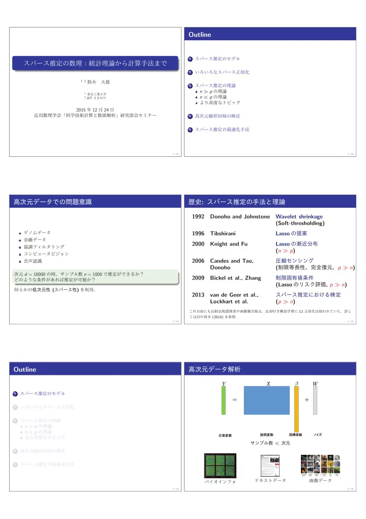
95 / 95