Outline Motivation (1/2) Suppose that data X was randomly generated - - PDF document

SLIDE 1

1

1

Non-Gaussian Methods for Learning Linear Structural Equation Models

UAI2010 Tutorial, Catalina Island

1

Equation Models

Shohei Shimizu and Yoshinobu Kawahara

Osaka University Special thanks to Aapo Hyvärinen, Patrik O. Hoyer and Takashi Washio.

2

Abstract

• Linear structural equation models (linear SEMs)

can be used to model data generating processes

• f variables.
• We review a new approach to learn or estimate

We review a new approach to learn or estimate linear structural equation models.

• The new estimation approach utilizes

non-Gaussianity of data for model identification and uniquely estimates much wider variety of models.

3

Outline

• Part I. Overview (70 min.) : Shohei
• Break (10 min.)
• Part II. Recent advances (40 min): Yoshi

– Time series – Latent confounders

4

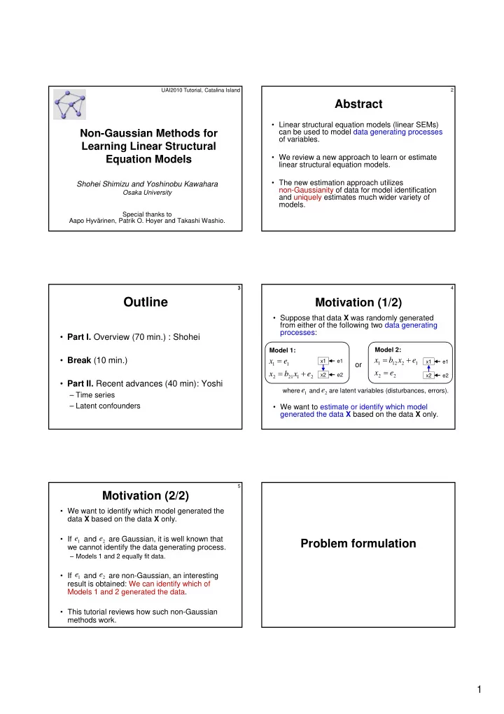
Motivation (1/2)

• Suppose that data X was randomly generated

from either of the following two data generating processes:

Model 1: Model 2: where and are latent variables (disturbances, errors).

• We want to estimate or identify which model

generated the data X based on the data X only.

• r

2 1 21 2 1 1

e x b x e x   

2 2 1 2 12 1

e x e x b x   

x1 x2 e1 e2 x1 x2 e1 e2

1

e

2

e

5

Motivation (2/2)

• We want to identify which model generated the

data X based on the data X only.

• If x1 and x2 are Gaussian, it is well known that

we cannot identify the data generating process.

M d l 1 d 2 ll fit d t

1

e

2

e

– Models 1 and 2 equally fit data.

• If x1 and x2 are non-Gaussian, an interesting

result is obtained: We can identify which of Models 1 and 2 generated the data.

• This tutorial reviews how such non-Gaussian

methods work.

1

e

2

e

Problem formulation

SLIDE 2

2

7

Basic problem setup (1/3)

• Assume that the data generating process of

continuous observed variables is graphically represented by a directed acyclic graph (DAG).

– Acyclicity means that there are no directed cycles. E l f di t d

i

x

x3 x1 e3 e1 x2 e2 x3 x1 e3 e1 x2 e2

Example of a directed acyclic graph (DAG): Example of a directed cyclic graph:

is a parent of etc.

1

x

3

x

8

Basic problem setup (2/3)

• Further assume linear relations of variables .
• Then we obtain a linear acyclic SEM (Wright, 1921; Bollen,

1989):

e Bx x  

i j ij i

e x b x  



• r

i

x

where – The are continuous latent variables that are not determined inside the model, which we call external influences (disturbances, errors). – The are of non-zero variance and are independent. – The ‘path-coefficient’ matrix B = [ ] corresponds to a DAG. i i j j ij i



• f

parents :

i

e

i

e

ij

b

9

• A three-variable linear acyclic SEM:

Example of linear acyclic SEMs

                                          

3 2 1 3 2 1 3 2 1

3 . 1 5 . 1 e e e x x x x x x

2 1 2 1 3 1

3 . 1 5 . 1 e x e x x e x x      

• r
• B corresponds to the data-generating DAG:

      

x3 x1 e3 e1 x2 e2 1.5

• 1.3

B

3 3

e x 

i j ij

x x b to from edge directed No 0  

i j ij

x x b to from edge directed A 0  

10

                         

1 3 1 3 1 3

5 . 1 e e x x x x

Assumption of acyclicity

• Acyclicity ensures existence of an ordering of

variables that makes B lower-triangular with zeros on the diagonal.

i

x

                          

2 1 2 1 2 1

3 . 1 5 . 1 e e x x x x                         

2 2 2

3 . 1 e x x       

x3 x1 e3 e1 x2 1.5

• 1.3

perm

B

e2

                       

3 2 3 2 3 2

e x x       

B

. versa vice not but , ,

• f

ancestor an be may . : is

• rdering

The

2 1 3 2 1 3

x x x x x x  

11

Assumption of independence between external influences

• It implies that there are no latent confounders

(Spirtes et al. 2000)

– A latent confounder is a latent variable that is a parent of more than or equal to two observed variables:

f

• Such a latent confounder makes external influences

dependent (Part II):

x1 x2

f

e1’ e2’

x1 x2 e1 e2

f

• Assume that data X is randomly sampled

from a linear acyclic SEM (with no latent confounders):

12 12

Basic problem setup (3/3): Learning linear acyclic SEMs

• Goal: Estimate the path-coefficient matrix B by
• bserving data X only!

– B corresponds to the data-generating DAG.

e Bx x  

x1 x2 e1 e2

21

b

SLIDE 3

3

Problems:

Identifiability problems of con entional methods conventional methods

14 14

Under what conditions B is identifiable?

• `B is identifiable’ `B is uniquely determined or

estimated from p(x)’.



• Linear acylic SEM:

– B and p(e) induce p(x). – If p(x) are different for different B, then B is uniquely determined.

e Bx x  

x1 x2 e1 e2

21

b

15

Conventional estimation principle: Causal Markov condition

• If the data-generating model is a linear

acyclic SEM, causal Markov condition holds :

E h b d i bl i i i d d t f it – Each observed variable xi is independent of its non-descendants in the DAG conditional on its parents (Pearl & Verma, 1991) :

   







p i i i

x x p p

1

• f

parents | x

i

x

16 16

Conventional methods based on causal Markov condition

• Methods based on conditional independencies

(Spirtes & Glymour, 1991)

– Many linear acyclic SEMs give a same set of conditional independences and equally fit data.

• Scoring methods based on Gaussianity

(Chickering, 2002)

– Many linear acyclic SEMs give a same Gaussian distribution and equally fit data.

• In many cases, path-coefficient matrix B is not

uniquely determined.

17 17

• Two models with Gaussian e1 and :

Example

2 1 2 1 1

8 . e x x e x   

2 2 1 2 1

8 . e x e x x   

Model 1: Model 2:

x1 x2 e1 e2 x1 x2 e1 e2

1

e

2

e

• Both introduce no conditional independence:
• Both induce the same Gaussian distribution:

 

8 . , cov

2 1

  x x

                          1 8 . 8 . 1 ~

2 1

N x x

   

1 var var

2 1

  x x

   

,

2 1

  e E e E

A solution: Non-Gaussian approach pp

SLIDE 4

4

19 19

A new direction: Non-Gaussian approach

• Non-Gaussian data in many applications:

– Neuroinformatics (Hyvarinen et al., JMLR, 2001); Bioinformatics (Sogawa et al., ICANN2010); Social sciences (Micceri, 1989); Economics (Moneta, Entner, et al., 2010)

• Utilize non-Gaussianity for model identification.

– Bentler (Psychometrika, 1983)

• The path-coefficient matrix B is uniquely

estimated if ei are non-Gaussian.

– Shimizu, Hoyer, Hyvarinen & Kerminen (JMLR, 2006) i

e

20 20

Illustrative example: Gaussian vs non-Gaussian

Gaussian Non-Gaussian (uniform) Model 1:

x1

e1

x1 x2 x1 x2 1 1

8 e x  

Model 2:

x1 x2

x2

e2

x1 x2

e1 e2

x1 x2 2 1 2

8 . e x x  

2 2 1 2 1

8 . e x e x x   

   

1 var var

2 1

  x x

   

,

2 1

  e E e E

21 21

• Non-Gaussian version of linear acyclic SEM:

Linear Non-Gaussian Acyclic Model: LiNGAM

(Shimizu, Hyvarinen, Hoyer & Kerminen, JMLR, 2006)

e Bx x  

e x b x  



• r

where – The external influence variables (disturbances, errors) are

• of non-zero variance.
• non-Gaussian and mutually independent.

i

e

e Bx x  

i i j j ij i

e x b x  



• f

parents :

• r

22

Identifiability of LiNGAM model

• LiNGAM model can be shown to be

identifiable.

– B is uniquely estimated.

• To see the identifiability, helpful to review

independent component analysis (ICA)

(Hyvarinen et al., 2001).

23 23

Independent Component Analysis (ICA) (Jutten & Herault, 1991; Comon, 1994)

• Observed random vector x is modeled by

h

As x 







p j j ij i

s a x

1

• r

where – The mixing matrix A = [ ] is square and is of full column rank. – The latent variables (independent components) are non-Gaussian and mutually independent.

• Then, A is identifiable up to permutation P and

scaling D of the columns:

i

s APD A 

ica

ij

a

24 24

Estimation of ICA

• Most of estimation methods estimate

(Hyvarinen et al., 2001)

• Most of the methods minimize mutual information (or its

approximation) of estimated independent components:

:

1 

 A W

s W As x

1 

 

• W is estimated up to permutation P and scaling D of the rows:
• Consistent and computationally efficient algorithms:

– Fixed point (FastICA) (Hyvarinen,99); Gradient-based (Amari, 98) – Semiparametric: no specific distributional assumption

x W s

ica

 ˆ  

1 

  PDA PDW Wica

SLIDE 5

5

Back to LiNGAM model

26 26

Identifiability of LiNGAM (1/3): ICA achieves half of identification

• LiNGAM model is ICA.

– Observed variables are linear combinations of non-Gaussian independent external influences :

e B I x e Bx x



    

1

) (

i

x

i

e

• ICA gives .

– P: unknown permutation matrix – D: unknown scaling (diagonal) matrix

• Need to determine P and D to identify B.

e W Ae

1 

 

) ( B I PD PDW W   

ica 27 27

Identifiability of LiNGAM (2/3): No permutation indeterminacy (1/6)

• ICA gives .

– P : permutation matrix; D: scaling (diagonal) matrix

• We want to find such a permutation matrix that cancels the

permutation i e :

) ( B I PD PDW W   

ica

I P P  P P permutation , i.e., :

• We can show (Shimizu et al., UAI05) (illustrated in the next slides):

– If , i.e., no permutation is made on the rows of , has no zero in the diagonal (obvious by definition). – If , i.e., any nonidentical permutation is made on the rows

• f , has a zero in the diagonal.

I P P 

I P P 

ica

W P

I P P 

ica

W P

I 

DW PDW P W P  

ica

P

DW DW

28

Identifiability of LiNGAM (2/3):

No permutation indeterminacy (2/6)

• By definition

has all unities in the diagonal.

– The diagonal elements of B are all zeros.

• Acyclicity ensures existence of an ordering of variables

that makes lower triangular and then is

B I W   B I W B

that makes lower triangular, and then is also lower triangular.

• So, WLG,

can be assumed to be lower triangular:

           1 * * 1 * 1 W 0 0

No zeros in the diagonal!

B I W   B W

29

Identifiability of LiNGAM (2/3): No permutation indeterminacy (3/6)

• Premultiplying

by a scaling (diagonal) matrix D does NOT change the zero/non-zero pattern of :

W W

          

33 22 11

* * * d d d DW

           1 * * 1 * 1 W 0 0

No zeros in the diagonal!

30 30

Identifiability of LiNGAM (2/3): No permutation indeterminacy (4/6)

• Any other permutation of the rows of

changes the zero/non-zero pattern of and brings zero in the diagonal: DW DW

          

33 11 22 12

* * * d d d DW P           

33 22 11

* * * d d d DW

Exchanging 1st and 2nd rows Zero in the diagonal!

SLIDE 6

6

• Any other permutation of the rows of

changes the zero/non-zero pattern of and brings zero in the diagonal:

31 31

Identifiability of LiNGAM (2/3): No permutation indeterminacy (5/6)

DW DW

          

33 22 11

* * * d d d DW            * * *

11 22 33 13

d d d DW P

Exchanging 1st and 3rd rows Zero in the diagonal!

32 32

Identifiability of LiNGAM (2/3): No permutation indeterminacy (6/6)

• We can find correct by finding that gives no

zero on the diagonal of (Shimizu et al., UAI05).

ica

W P P P

• Thus, we can solve the permutation

indeterminacy and obtain:

 

B I D DW PDW P W P    

ica

I 

33 33

Identifiability of LiNGAM (3/3): No scaling indeterminacy

• Now we have:
• Then,

B) D(I W P  

ica

 

ica

W P D diag 

• Divide each row of by its corresponding

diagonal element to get , i.e., :

ica

W P

 

B I B) D(I D W P W P    

  1 1

diag

ica ica

B I  B

34 34

Estimation of LiNGAM model

• 1. ICA-LiNGAM algorithm
• 2. DirectLiNGAM algorithm

35 35

Two estimation algorithms

• ICA-LiNGAM algorithm

(Shimizu, Hoyer, Hyvarinen & Kerminen, JMLR, 2006)

• DirectLiNGAM algorithm

(Shimizu, Hyvarinen, Kawahara & Washio, UAI09)

• Both estimate an ordering of variables that makes

g the path-coefficient matrix B to be lower-triangular.

– Acyclicity ensures existence of such an ordering.

perm perm perm

e x x           

perm

B

O

x2 x3 x1 redundant edges A full DAG

36 36

Once such an ordering is found…

• Many existing methods can do:

– Pruning the redundant path-coefficients

• Sparse methods like weighted lasso (Zou, 2006）

– Finding significant path-coefficients

• Testing, bootstrapping (Shimizu et al., 2006; Hyvarinen et al. 2010)

x2 x3 x1 x2 x3 x1 perm perm perm

e x x           

perm

B

O

* * * *

A full DAG

SLIDE 7

7

37 37

• 1. Outline of ICA-LiNGAM algorithm

(Shimizu, Hoyer, Hyvarinen, & Kerminen, JMLR, 2006)

• 1. Estimate B by ICA

+ permutation

• 2. Pruning

Redundant edges

x3 x2 x1 x3 x3

23

b

13

b

x1 x2

38 38

1. Perform ICA (here, FastICA) to obtain an estimate of

ICA-LiNGAM algorithm (1/2): Step 1. Estimation of B

B) PD(I PDW W   

ica

2. Find a permutation that makes the diagonal elements of as large as possible in absolute value: 3. Normalize each row of , then we get an estimate of I-B and .

 

ii ica

W P P

P

ˆ 1 min ˆ 

ica

W P ˆ

Hungarian alg.

(Kuhn, 1955)

P

ica

W P ˆ ˆ B ˆ

39 39

ICA-LiNGAM algorithm (2/2): Step 2. Pruning

• Find such an ordering of variables that makes

estimated B be as close to be lower-triangular as possible.

– Find a permutation matrix Q that minimizes the sum of the elements in its upper triangular part: elements in its upper triangular part: – Approximate algorithm for large variables (Hoyer et al., ICA06)

 







j i ij T 2

ˆ min ˆ Q B Q Q

Q

x3 x2 x1 x3 x3

0.1 0.1

3

0.1 0.1 3 5 5

• 0.01

x1 x2

40 40

Basic properties

• f ICA-LiNGAM algorithm
• ICA-LiNGAM algorithm = ICA + permutations

– Computationally efficient with the help of well-developed ICA techniques.

• Potential problems

– ICA is an iterative search method:

• May get stuck in a local optimum if the initial guess or step

size is badly chosen.

– The permutation algorithms are not scale-invariant:

• May provide different estimates for different scales of

variables.

Estimation of LiNGAM model

41

• 1. ICA-LiNGAM algorithm
• 2. DirectLiNGAM algorithm

42 42

• 2. DirectLiNGAM algorithm

(Shimizu, Hyvarinen, Kawahara & Washio, UAI2009)

• Alternative estimation method without ICA

– Estimates an ordering of variables that makes path- coefficient matrix B to be lower triangular.

 

A full DAG

• Many existing methods can do further pruning or

finding significant path coefficients (Zou, 2006;

Shimizu et al., 2006; Hyvarinen et al. 2010)

perm perm perm

e x x           

perm

B

O

x2 x3 x1 Redundant edges A full DAG

SLIDE 8

8

43

Basic idea (1/2) :

An exogenous variable can be at the top of a right ordering

• An exogenous variable

is a variable with no parents (Bollen, 1989), here .

The corresponding row of B has all zeros

j

x

3

x

– The corresponding row of B has all zeros.

• So, an exogenous variable can be at the top of

such an ordering that makes B lower triangular.

                                          

2 1 3 2 1 3 2 1 3

3 . 1 5 . 1 e e e x x x x x x x3 x1 x2

44

Basic idea (2/2): Regress exogenous

• ut
• Compute the residuals regressing the
• ther variables on exogenous

:

– The residuals form a LiNGAM model. – The ordering of the residuals is equivalent to that of corresponding original variables 3

x

 

) 2 , 1 (

3

 i r

i 3

x

) 2 , 1 (  i xi

corresponding original variables.

• Exogenous implies ` can be at the second top’.

) 3 ( 1

r

1

x

                                          

2 1 3 2 1 3 2 1 3

3 . 1 5 . 1 e e e x x x x x x                           

2 1 ) 3 ( 2 ) 3 ( 1 ) 3 ( 2 ) 3 ( 1

3 . 1 e e r r r r

) 3 ( 2

r

) 3 ( 1

r

x3 x1 x2

45

• Iteratively find exogenous variables until all the

variables are ordered:

• 1. Find an exogenous variable .

– Put at the top of the ordering. – Regress out.

2 Fi d id l h

Outline of DirectLiNGAM

3

x

) 3 (

r

3

x

3

x

• 2. Find an exogenous residual, here .

– Put at the second top of the ordering. – Regress out.

• 3. Put at the third top of the ordering and terminate.

The estimated ordering is

) ( 1

r

) 3 ( 2

r

) 3 ( 1

r

x3 x1 x2

) 1 , 3 ( 2

r

1

x

) 3 ( 1

r

2

x .

2 1 3

x x x  

• Step. 1
• Step. 2
• Step. 3

46-1

Identification of an exogenous variable (two variable cases)

ii) is NOT exogenous

i)

is exogenous

 

21 2 1 21 2 1 1

    b e x b x e x

) (

1 1

e x 

1

x

 

2 2 12 2 12 1

e x b x b x    

1

e

 

) var( var ) var( ) , cov( 1 ) var( ) , cov( ,

• n

Regressing

1 2 12 2 1 1 2 12 1 1 1 2 2 ) 1 ( 2 2 1

x x b x x x x b x x x x x r x x           

2 1 21 2 1 1 1 2 2 ) 1 ( 2 1 2

) var( ) , cov( ,

• n

Regressing e x b x x x x x x r x x     

t independen NOT are and

) 1 ( 2 1

r x t independen are and

) 1 ( 2 1

r x

1

e

Darmoir-Skitovitch’ theorem:

Define two variables and as

46-2

Need to use Darmoir-Skitovitch’ theorem (Darmois, 1953)

ii) is NOT exogenous

1

x

 

2 2 12 1 2 12 1

e x b e x b x     

 

 

p j j p j j

e a x e a x

2 2 1 1

,

1

x

2

x 1

 

1 1 2 2 1 1 2 12 1 1 1 2 2 ) 1 ( 2 2 1

) var( var ) var( ) , cov( 1 ) var( ) , cov( ,

• n

Regressing e x x x x x x b x x x x x r x x           

t independen NOT are and

) 1 ( 2 1

r x

 

  j j j j j j 1 2 2 1 1 1

where are independent random variables. If there exists a non-Gaussian for which , and are dependent.

j

e

i

e

2 1



i ia

a

1

x

2

x

12

b

47

• Lemma 1:

and its residual are independent for all is exogenous

Identification of an exogenous variable (More than 2 variable cases)

 

j j j i i j i

x x x x x r ) var( ) cov(

,

 

j

x j i 

j

x 

are independent for all is exogenous

• In practice, we can identify an exogenous variable

by finding a variable that is most independent of its residuals. j i 

j

x 

SLIDE 9

9

• Evaluate independence between a variable and a

residual by a nonlinear correlation:

• Taking the sum over all the residuals we get:

48

Independence measures

    



tanh , corr

) (

 g r g x

j i j

• Taking the sum over all the residuals, we get:
• Can use more sophisticated measures as well

(Bach & Jordan, 2002; Gretton et al., 2005; Kraskov et al., 2004).

– Kernel-based independence measure (Bach & Jordan, 2002)

• ften gives more accurate estimates (Sogawa et al., IJCNN10).

       





 

j i j i j j i j

r x g r g x T

) ( ) (

, corr , corr

49

Important properties of DirectLiNGAM

• DirectLiNGAM repeats:

– Least squares simple linear regression – Evaluation of pairwise independence between each variable and its residuals variable and its residuals

• No algorithmic parameters like stepsize, initial

guesses, convergence criteria

• Guaranteed convergence in a fixed number of

steps (the number of variables)

50

Estimation of LiNGAM model: Summary (1)

• Two estimation algorithms:

– ICA-LiNGAM: Estimation using ICA

• Pros. Fast
• Cons Possible local optimum; Not scale invariant
• Cons. Possible local optimum; Not scale-invariant

– DirectLiNGAM: Alternative estimation without ICA

• Pros. Guaranteed convergence; Scale-invariant
• Cons. Less fast

– Cf. Neither needs faithfulness (Shimizu et al., JMLR,

2006; Hoyer, personal comm., July, 2010).

51

• Experimental comparison of the two algorithms:

(Sogawa et al., IJCNN2010)

• Scalability: Both can analyze 100 variables. The

performances depend on the sample size etc., of course! S l i B th d t l t 1000 l i f

Estimation of LiNGAM model: Summary (2)

• Sample size: Both need at least 1000 sample size for

more than 10 variables.

• Scale invariance: ICA-LiNGAM is less robust for changing

scales of variables.

• Local optima?:

– For less than 10 variables, ICA-LiNGAM often a bit better. – For more than 10 variables, DirectLiNGAM often better perhaps because the problem of local optima becomes more serious?

52

Testing and Reliability evaluation y

53

Testing testable assumptions

• Non-Gaussianity:

– Gaussianity tests

• Could detect violations of some assumptions:

– Local test

• Independence of external influences
• Conditional independencies between observed

variables (causal Markov condition)

• Linearity

– Overall fit of the model assumptions

• Chi-square test using 3rd and/or 4th-order moments

(Shimizu & Kano, 2008)

• Still under development

i

e

i

x

SLIDE 10

10

54

Reliability evaluation

• Need to evaluate statistical reliability of LiNGAM

results:

– Sample fluctuations – Smaller non-Gaussianity makes the model closer to be NOT identifiable.

• Reliability evaluation by bootstrapping:

(Komatsu et al., ICANN2010)

– If either the sample size is too small or the magnitude

• f non-Gaussianity is too small, LiNGAM would give

very different results for bootstrap samples.

55

Extensions

56

Extensions (a partial list)

• Relaxing the assumptions of LiNGAM model:

– Acyclic  Cyclic (Lacerda et al., UAI2008) – Single homogenous population  heterogeneous population (Shimizu et al., 2007) – i.i.d. sampling  time structures (Part II.) (Hyvarinen et al, – No latent confounders  Allow latents (Part II.) (Hoyer et al., – Linear  non-linear (Hoyer et al., NIPS08; Zhang & Hyvarinen, UAI09;

Tilmann & Spirtes, NIPS09)

JMLR,2010, Kawahara, S et al., 2010) IJAR, 08; Kawahara, Bollen et al., 2010)

57

Application areas so far

58

Non-Gaussian SEMs have been applied to…

• Neuroinformatics

– Brain connectivity analysis

(Hyvarinen et al., JMLR, 2010; Zhang & Hyvarinen, UAI 2010.)

• Bioinformatics

Gene network estimation (Sogawa et al

ICANN2010)

– Gene network estimation (Sogawa et al., ICANN2010)

• Economics (Wan & Tan, 2009; Moneta, Entner, Hoyer & Coad, 2010)
• Genetics (Ozaki & Ando, 2009)
• Environmental sciences (Niyogi et al., 2010)
• Physics (Kawahara, Shimizu & Washio, 2010)
• Sociology (Kawahara, Bollen, Shimizu & Washio, 2010)

59

Final summary of Part I

• Use of non-Gaussianity in linear SEMs is

useful for model identification.

• Non-Gaussian data is encountered in many

applications applications.

• The non-Gaussian approach can be a good
• ption.
• Links to codes and papers:

http://homepage.mac.com/shoheishimizu/lingampapers.html

SLIDE 11

11

60

FAQs

61

• Q. My data is Gaussian.

LiNGAM will not be useful.

• A. You’re right. Try Gaussian methods.
• Comment: Hoyer et al. (UAI2008) showed:

`To hat e tent one can identif the model for a To what extent one can identify the model for a mixture of Gaussian and non-Gaussian external influence variables’.

62

• Q. I applied LiNGAM, but the result is not

reasonable to background knowledge.

• A. You might first want to check:

– Some model assumptions might be violated.  Try other extensions of LiNGAM

• r non-parametric methods PC or FCI etc
• r non parametric methods PC or FCI etc.

(Spirtes et al., 2000).

– Small sample size or small non-Gaussianity  Try bootstrap to see if the result is reliable. – Background knowledge might be wrong.

63

• Q. Relation to causal Markov

condition?

• A. The following 3 estimation principles are

equivalent (Zhang & Hyvarinen, ECML09; Hyvarinen et al., JMLR, 2010):

• 1. Maximize independence between external influences .

2 Minimize the sum of entropies of external influences

i

e e

• 2. Minimize the sum of entropies of external influences .
• 3. Causal Markov condition (Each variable is independent of

its non-descendants in the DAG conditional on its parents) AND maximization of independence between the parents of each variable and its corresponding external influences .

i

e

i

e

64

• Q. I am a psychometrician and am

more interested in latent factors.

• A. Shimizu, Hoyer, and Hyvarinen. (2009)

proposes LiNGAM for latent factors:

d Bf f  

• - LiNGAM for latent factors

e Gf x  

• - Measurement model

65

• Q. Prior knowledge?

– It is possible to incorporate prior knowledge. The accuracy of DirectLiNGAM is often greatly improved even if the amount of prior knowledge is not so large (Inazumi et al., LVA/ICA2010).

• Q. Sparse LiNGAM?

– Zhang et al. (ICA09) and Hyvarinen et al. (JMLR, 2010). – ICA + adaptive Lasso (Zou 2006)

Others

ICA + adaptive Lasso (Zou, 2006).

• Q. Bayesian approach?

– Hoyer and Hyttinen (NIPS08); Henao et al. (NIPS09).

• Q. The idea can be applied to discrete variables?

– One proposal by Peters et al. (AISTATS2010). – Comment: if your discrete variables are close to be continuous, e.g.,

• rdinal scales with many points, LiNGAM might work.

SLIDE 12

12

66

• A. Several nonlinear SEMs have been proposed:

– DAG; No latent confounders.

• Q. Nonlinear extensions?

 

i j i ij i

e x j f x   

• f

parent

• - Imoto et al. (2002)

1.

• For two variable cases, unique identification possible

except several combinations of nonlinearities and distributions (Hoyer et al., NIPS08; Zhang & Hyvarinen, UAI09).

   

 

i i i i i i i i i j

e x f f x e x f x    



• f

parents

• f

parents

1 , 1 2 ,

• - Hoyer et al. (NIPS08)
• - Zhang et al. (UAI09)

2. 3.

67

• Proposals to aim at computational efficiency (Mooij et al.,

ICML09; Tilmann & Spirtes, NIPS09; Zhang & Hyvarinen, ECML09;UAI09).

• Pros:

– Nonlinear models are more general than linear models.

Nonlinear extensions (continued)

g

• Cons:

– Computationally demanding.

• Current: at most 7 or 8 variables.
• Perhaps, assumption of Gaussian external influences might help.

– Imoto et al. (2002) analyzes 100 variables.

– More difficult to allow other possible violations of LiNGAM assumptions, latent confounders etc.

68

• A. Try non-parametric methods, e.g.,

– DAG: PC (Spirtes & Glymour, 1991) – DAG with latent confounders: FCI (Spirtes et al

1995)

• Q. My data follows neither such linear

SEMs nor such nonlinear SEMs as you have talked.

– DAG with latent confounders: FCI (Spirtes et al., 1995).

• Probably you get an (probably large)

equivalence class rather than a single model, but that would be the best you currently can.

 

i i i i

e x f x ,

• f

parents 

69

• Q. Deterministic relations?
• A. LiNGAM is not applicable.
• See Daniusis et al. (UAI2010) for a method to

analyze deterministic relations analyze deterministic relations.