Outline Introduction TSV Array Cross Talk Analysis Return Path - PDF document

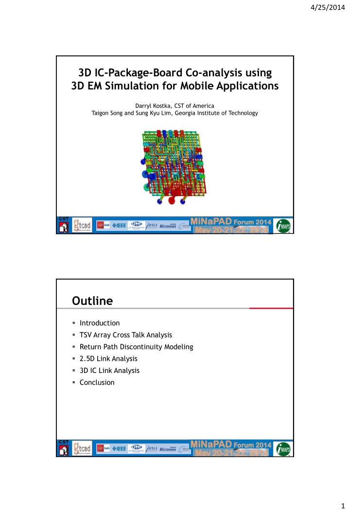
4/25/2014 3D IC-Package-Board Co-analysis using 3D EM Simulation for Mobile Applications Darryl Kostka, CST of America Taigon Song and Sung Kyu Lim, Georgia Institute of Technology CST – COMPUTER SIMULATION TECHNOLOGY | www.cst.com ECTC 2013 Outline  Introduction  TSV Array Cross Talk Analysis  Return Path Discontinuity Modeling  2.5D Link Analysis  3D IC Link Analysis  Conclusion CST – COMPUTER SIMULATION TECHNOLOGY | www.cst.com ECTC 2013 1

4/25/2014 Introduction to 3D Integration System-on- System-in- Chip (SoC) Package (SiP) Source: Cadence Design Systems, Inc. “3D ICs with TSVs— Design Challenges and Requirements” 3D IC 2.5D Stacking CST – COMPUTER SIMULATION TECHNOLOGY | www.cst.com ECTC 2013 TSV Signal-Ground Pair Insertion Loss (dB) D=100 μ m, R=15 μ m, L=100 μ m, Sharp slope due to d ox =0.1 μ m, ε SiO2 =3.9 (tand=0.001), Losses due to transition from slow wave ε Si =11.9 (cond=10S/m) displacement to quasi-TEM mode currents in Si CST – COMPUTER SIMULATION TECHNOLOGY | www.cst.com ECTC 2013 2

4/25/2014 Cross Talk: TSV Array 1 Aggressor via 2 Neighboring Victim via 3 Shielded Victim via Return vias Victim vias  5x5 TSV array with 1 driven aggressor and two victim vias;  Aggressor (TSV1) is driven with a pulse (risetime=100ps, amplitude=2V) using a 50Ohm source resistor.  Far end of aggressor TSV and both sides of all other signal TSVs are terminated in 50Ohms Baseline: D=100 μ m, R=10 μ m, L=200 μ m, d ox =1 μ m, ε SiO2 =3.9 (0.001), ε Si =11.9 (10S/m) CST – COMPUTER SIMULATION TECHNOLOGY | www.cst.com ECTC 2013 Cross Talk: TSV Array NEXT – Frequency domain NEXT – Time domain Neighboring victim Shielded victim  Thicker oxide liners help reduce cross talk for low resistivity substrates  High resistivity substrates act as low loss dielectrics and therefore help reduce cross talk  Low resistivity substrate has a larger peak voltage and longer coupled noise duration (ISI)  Chip-package co-design since TSV response in the chip stack can propagate into package CST – COMPUTER SIMULATION TECHNOLOGY | www.cst.com ECTC 2013 3

4/25/2014 Interposer: Return Path Discontinuities  Microstrip-to-microstrip transition causes a change in the reference plane (RPD)  Results in large SSN voltage induced between planes at resonance frequencies  Increased insertion loss Surface current distribution (Glass) @30GHz showing cavity resonance CST – COMPUTER SIMULATION TECHNOLOGY | www.cst.com ECTC 2013 Eye Diagrams for Silicon and Glass Interposers Glass Silicon 3.2 Gbps 2 10 -1 PRBS stream 17.89p 6.7ps 0.29V 0.31V s 282.6p 295.2p s s  Jitter and eye opening are considerably improved in the Silicon interposer, in comparison with the Glass interposer  Performance of glass interposer can be improved by using decoupling capacitors CST – COMPUTER SIMULATION TECHNOLOGY | www.cst.com ECTC 2013 4

4/25/2014 2.5D Link Test Case Signal Signal Die size: 1 mm x 1 mm, 250 um thickness (Die 1 is identical to Die 2) Double Sided Silicon Interposer size: 40 mm x 40 mm, 300 um thickness u-bump dimensions: 60 um diameter , 52 um height, 200 um pitch TPV dimensions: 40 um diameter , 300 um height, 200 um pitch CST – COMPUTER SIMULATION TECHNOLOGY | www.cst.com ECTC 2013 IC Design I/O Pad Map GDSII Import from Cadence Virtuoso Silicon IC BEOL M1 M10  NCSU FreePDK 45nm technology library u-bump  10 metal layers, 12um thick Cu backend  11 signals total CST – COMPUTER SIMULATION TECHNOLOGY | www.cst.com ECTC 2013 5

4/25/2014 Double Sided Silicon Interposer Design Interposer IC 1 IC 2 20mm Microstrip-to-microstrip signal routing used to maximize RPD 40mm effects (worst case scenario) (Eps = 2.51, tanD = 0.004) CST – COMPUTER SIMULATION TECHNOLOGY | www.cst.com ECTC 2013 2.5D Link: Analysis Methodology I Method 1: Complete chip-interposer-chip link co-simulation  Pos: Highest level of accuracy since all 3D coupling effects between the ICs and interposer are captured  Neg: Not computationally feasible (3D full-wave analysis) due to the complexity of the IC design and the aspect ratios involved CST – COMPUTER SIMULATION TECHNOLOGY | www.cst.com ECTC 2013 6

4/25/2014 2.5D Link: Analysis Methodology II Method 2: Decoupling / Cascading approach Reference Plane  Center of the u-bump array is used as the reference plane (electric wall)  All signal, power and ground nets need to be terminated to maintain return current path continuity Electric Wall used as Discrete Port Reference + port Electric Wall used as Discrete Port Reference S-parameters S-parameters S-parameters (Die 1) (Interposer) (Die 2) CST – COMPUTER SIMULATION TECHNOLOGY | www.cst.com ECTC 2013 2.5D Link: Analysis Methodology II IC PEC sheet reference Interposer PEC sheet reference CST – COMPUTER SIMULATION TECHNOLOGY | www.cst.com ECTC 2013 7

4/25/2014 2.5D Link: Analysis Methodology III Method 2: Decoupling / Cascading approach Reference Plane Reference Plane The reference plane is selected along a uniform section of the signal traces to ensure TEM propagation mode. CST – COMPUTER SIMULATION TECHNOLOGY | www.cst.com ECTC 2013 Excitation Port Definition Die 1 Die 2 Port 7 Port 5 Port 3 Port 1 Port 4 Port 2 Port 8 Port 6 Die 1 and Die 2 are identical CST – COMPUTER SIMULATION TECHNOLOGY | www.cst.com ECTC 2013 8

4/25/2014 IC: Surface Current Distribution 100 MHz 2 GHz Signal Excitation Port Signal Excitation Port Coupling to surrounding (non neighboring) nets can be observed at higher frequencies CST – COMPUTER SIMULATION TECHNOLOGY | www.cst.com ECTC 2013 S-Parameter Results Port 5 Port 7 RL … Port 1 Port 3 Port 2 … Port 4 … Port 6 … Port 8 IL  For the “fewer pins” case, FEXT only the PWR/GND pins neighboring the signal pins were included  Results demonstrate that good correlation can be achieved provided the return current path continuity is NEXT preserved CST – COMPUTER SIMULATION TECHNOLOGY | www.cst.com ECTC 2013 9

4/25/2014 3D IC Link Test Case Signal Signal Die size: 1 mm x 1 mm, 250 um thickness Tier 3 = Signal I/Os, PDN distributed between Tier 2 and Tier 1 Double Sided Silicon Interposer size: 40 mm x 40 mm, 300 um thickness u-bump: 36 um diameter , 200 um pitch flip-chip bump: 60um diameter TSV: 12 um diameter , 50 um height TPV: 40 um diameter , 300 um height CST – COMPUTER SIMULATION TECHNOLOGY | www.cst.com ECTC 2013 3D IC Link: Analysis Methodology Full 3D link Method A Method B Method C  Center of the u-bump and flip-chip bump arrays are used for the reference plane locations  All signal, power and ground nets are terminated to maintain return current path continuity CST – COMPUTER SIMULATION TECHNOLOGY | www.cst.com ECTC 2013 10

4/25/2014 S-Parameter Results IL RL  Stronger coupling between TSV’s is observed in 3D IC’s and therefore using a decoupling simulation strategy NEXT provides inaccurate results FEXT especially for cross talk. CST – COMPUTER SIMULATION TECHNOLOGY | www.cst.com ECTC 2013 Conclusion  Demonstrated 3D full-wave electromagnetic analysis of a chip to chip channel using a simple IC (few I/O’s) and Si interposer prototype  TSV’s demonstrate high levels of cross talk due to the conductive Silicon substrate  For 2.5D applications, it is possible to decouple the IC from the interposer and obtain accurate results up to around 20 GHz  For 3D IC applications, the strong coupling between the TSV’s in the IC stack makes it impossible to perform a decoupled analysis CST – COMPUTER SIMULATION TECHNOLOGY | www.cst.com ECTC 2013 11