Outline Last time: Model-based recognition wrap-up Lecture 17: - PDF document

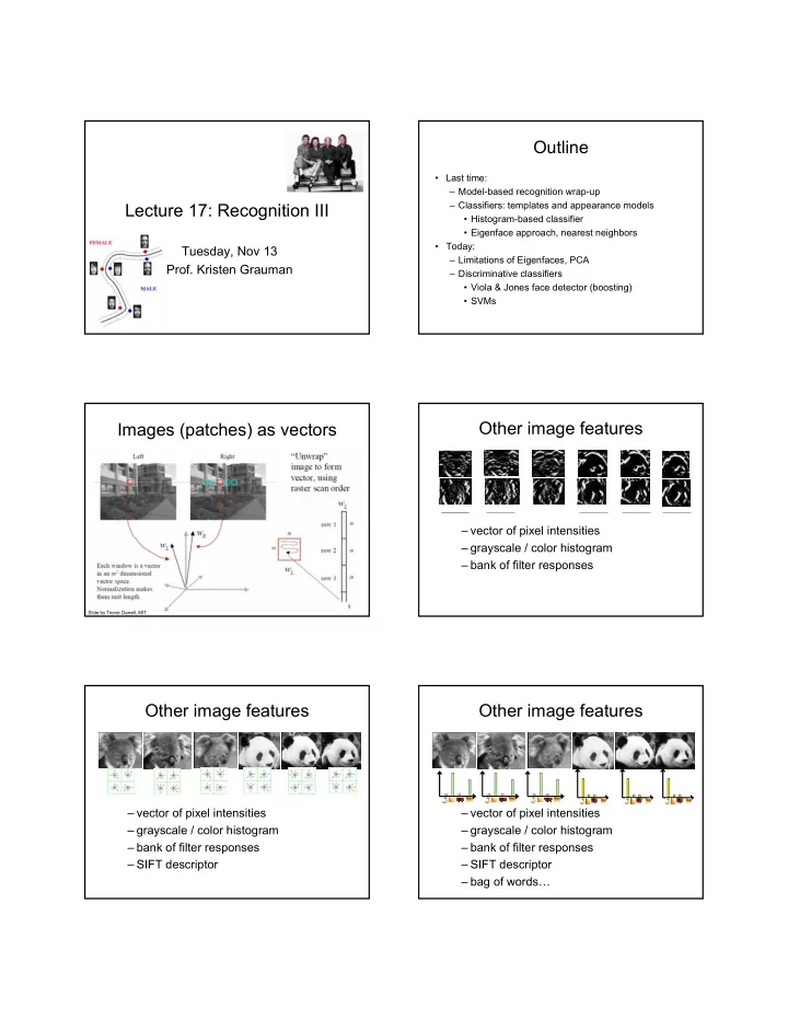
Outline • Last time: – Model-based recognition wrap-up Lecture 17: Recognition III – Classifiers: templates and appearance models • Histogram-based classifier • Eigenface approach, nearest neighbors • Today: Tuesday, Nov 13 – Limitations of Eigenfaces, PCA Prof. Kristen Grauman – Discriminative classifiers • Viola & Jones face detector (boosting) • SVMs Other image features Images (patches) as vectors – vector of pixel intensities – grayscale / color histogram – bank of filter responses Slide by Trevor Darrell, MIT Other image features Other image features – vector of pixel intensities – vector of pixel intensities – grayscale / color histogram – grayscale / color histogram – bank of filter responses – bank of filter responses – SIFT descriptor – SIFT descriptor – bag of words…

Feature space / Representation Last time: Eigenfaces u 1 • Construct lower Pixel value 2 Feature dimension 2 dimensional linear subspace that best explains variation of the training examples Pixel value 1 A face image A (non-face) image Feature dimension 1 Last time: Eigenfaces Last time: Eigenfaces • Premise: set of faces lie in a subspace of set of all images Training d = num rows * • Use PCA to determine the k ( k < d ) images: num cols in vectors u 1 ,… u k that span that training images subspace: x 1 ,…,x N x =~ μ + w 1 u 1 + … + w k u k • Then use nearest neighbors in “face space” coordinates (w 1 ,…w k ) to do recognition Last time: Eigenfaces Last time: Eigenfaces Top eigenvectors Face x in “face space” coordinates [ w 1 ,…, w k ]: of the covariance project the vector of pixel intensities onto each matrix: u 1 ,… u k eigenvector. Mean: μ u Pixel value 2 1 Pixel value 1

Last time: Eigenface recognition Last time: Eigenfaces • Process labeled training images: Reconstruction from low-dimensional – Unwrap the training face images into vectors to projection: form a matrix Reconstructed – Perform principal components analysis (PCA): face vector compute eigenvalues and eigenvectors of the covariance matrix + = – Project each training image onto subspace + + + + + + • Given novel image: – Project onto subspace – If Original face Unknown, not face vector – Else Classify as closest training face in k-dimensional subspace Benefits Limitations • PCA useful to represent data, but directions • Form of automatic feature selection of most variance not necessarily useful for • Can sometimes remove lighting variations classification • Computational efficiency: – Reducing storage from d to k – Distances computed in k dimensions Alternative: Fisherfaces Limitations Belhumeur et al. PAMI • PCA useful to represent data, but directions 1997 of most variance not necessarily useful for classification Rather than maximize • Not appropriate for all data: PCA is fitting scatter of projected Gaussian where Σ is covariance matrix classes as in PCA, maximize ratio of between-class scatter to within-class scatter by using Fisher’s Linear Discriminant There may be non-linear structure in high-dimensional data. Figure from Saul & Roweis

Limitations Prototype faces • PCA useful to represent data, but directions • Mean face as average of intensities: of most variance not necessarily useful for ok for well-aligned images… classification • Not appropriate for all data: PCA is fitting Gaussian where Σ is covariance matrix • Assumptions about pre-processing may be unrealistic, or demands good detector Mean: μ Prototype faces in shape and appearance Prototype faces …but unaligned shapes are a problem. 1 2 Mark coordinates Compute average shape for a group of faces of standard features 3 Warp faces to mean shape. Blend images to provide image Compare to faces that are blended without changing shape. with average appearance of the group, normalized for shape. We must include appearance AND shape to construct a prototype. University of St. Andrews, Perception Laboratory Figures from http://perception.st-and.ac.uk/Prototyping/prototyping.htm Using prototype faces: aging Using prototype faces: aging Enhance their differences to form caricature Average appearance Caricature and shape for different age groups. Shape differences for 25-29 yr olds and 50- 54 yr olds Burt D.M. & Perrett D.I. (1995) Perception of age in adult Caucasian male faces: computer graphic manipulation of shape and Burt D.M. & Perrett D.I. (1995) Perception of age in adult Caucasian male faces: computer graphic manipulation of shape and colour information. Proc. R. Soc. 259, 137-143. colour information. Proc. R. Soc. 259, 137-143.

Aging demo Using prototype faces: aging Input “feminize” “Facial aging”: get facial prototypes from different age groups, consider the difference to get function that maps one age group to another. University of St. Andrews, Perception Laboratory Child Teenager Older adult Baby • http://morph.cs.st-andrews.ac.uk//Transformer/ Burt D.M. & Perrett D.I. (1995) Perception of age in adult Caucasian male faces: computer graphic manipulation of shape and colour information. Proc. R. Soc. 259, 137-143. Aging demo Outline • Last time: Input “Masculinize” – Model-based recognition wrap-up – Classifiers: templates and appearance models • Histogram-based classifier • Eigenface approach, nearest neighbors • Today: – Limitations of Eigenfaces, PCA – Discriminative classifiers • Viola & Jones face detector (boosting) • SVMs Baby Teenager Older adult Child • http://morph.cs.st-andrews.ac.uk//Transformer/ Learning to distinguish faces and “non-faces” • How should the decision be made at every sub-window? Feature dimension 2 Feature dimension 1

Learning to distinguish faces and Questions “non-faces” • How should the decision be made at every • How to discriminate faces and non-faces? sub-window? – Representation choice • Compute boundary that divides the training – Classifier choice examples well… • How to deal with the expense of such a FACE NON-FACE windowed scan? Feature dimension 2 – Efficient feature computation – Limit amount of computation required to make a decision per window Feature dimension 1 [CVPR 2001] Value at (x,y) is Value at (x,y) is sum of pixels sum of pixels above and to the above and to the left of (x,y) left of (x,y) Defined as: Defined as: Can be computed in one pass over the original image:

Large library of filters Boosting • Weak learner : classifier with accuracy that need be only better than chance – Binary classification: error < 50% • Boosting combines multiple weak classifiers to create accurate ensemble • Can use fast simple classifiers without 180,000+ possible features associated with each image sacrificing accuracy. subwindow…efficient, but still can’t compute complete set at detection time. AdaBoost [Freund & Schapire]: Intuition AdaBoost [Freund & Schapire]: Intuition Figure from Freund and Schapire Figure from Freund and Schapire AdaBoost AdaBoost [Freund & Schapire]: Intuition Start with Algorithm uniform weights on training [Freund & examples Schapire]: Evaluate weighted error for each feature, pick best. Incorrectly classified -> more weight Correctly classified -> less weight Final classifier is combination of the weak classifiers. Final classifier is combination of the weak ones, weighted according to error they had. Figure from Freund and Schapire

Boosting for feature selection • Want to select the single rectangle feature that best separates positive and negative examples (in terms of weighted error). = Optimal threshold that results in minimal misclassifications Image subwindow This dimension: output of a possible rectangle feature on faces and non-faces. First and second features selected by AdaBoost. First and second features selected by AdaBoost. Questions Attentional cascade • First apply smaller (fewer features, efficient) • How to discriminate faces and non-faces? classifiers with very low false negative rates. – Representation choice – accomplish this by adjusting threshold on boosted – Classifier choice classifier to get false negative rate near 0. • How to deal with the expense of such a • This will reject many non-face windows early, windowed scan? but make sure most positives get through. – Efficient feature computation • Then, more complex classifiers are applied to – Limit amount of computation required to get low false positive rates. make a decision per window • Negative label at any point � reject sub- window

Running the detector • Scan across image at multiple scales and locations • Scale the detector (features) rather than the input image – Note: does not change cost of feature computation An implementation is available in Intel’s OpenCV library.

Profile Detection More Results Train with profile views instead of frontal Viola 2003 Viola 2003 Paul Viola, ICCV tutorial Paul Viola, ICCV tutorial Profile Features Fast detection: Viola & Jones Key points: • Huge library of features • Integral image – efficiently computed • AdaBoost to find best combo of features • Cascade architecture for fast detection Viola 2003 Paul Viola, ICCV tutorial