Outline Markov networks (a.k.a. Markov random fields) Markov - PDF document

Outline • Markov networks (a.k.a. Markov random fields) Markov Networks • Reading: Michael Jordan, Graphical Models , Statistical Science (Special November 12, 2009 Issue on Bayesian Statistics), 19, 140- CS 486/686 155, 2004. University of Waterloo 2 CS486/686 Lecture Slides (c) 2009 P. Poupart Recall Bayesian networks Markov networks • Directed acyclic graph • Undirected graph Cloudy Cloudy • Arcs often interpreted • Arcs simply indicate as causal relationships direct correlations Sprinkler Rain Sprinkler Rain • Joint distribution: • Joint distribution: product of conditional dist normalized product of potentials Wet • Popular in computer vision and grass Wet grass natural language processing 3 4 CS486/686 Lecture Slides (c) 2009 P. Poupart CS486/686 Lecture Slides (c) 2009 P. 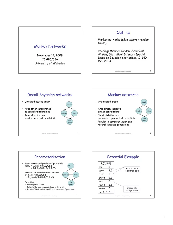Poupart Parameterization Potential Example f 1 (C,S,R) • Joint: normalized product of potentials Pr( X ) = 1/k Π j f j ( CLIQUE j ) Cloudy csr 3 = 1/k f 1 (C,S,R) f 2 (S,R,W) c~sr is more cs~r 2.5 likely than cs~r where k is a normalization constant c~sr 5 k = Σ X i Π j f j ( CLIQUE j ) Sprinkler Rain = Σ C,S,R,W f 1 (C,S,R) f 2 (S,R,W) c~s~r 5.5 ~csr 0 • Potential: Wet ~cs~r 2.5 – Non-negative factor grass – Potential for each maximal clique in the graph ~c~sr 0 impossible – Entries: “likelihood strength” of different configurations. configuration ~c~s~r 7 5 6 CS486/686 Lecture Slides (c) 2009 P. Poupart CS486/686 Lecture Slides (c) 2009 P. Poupart 1

Markov property Conditional Independence • Markov property: a variable is • X and Y are independent given Z iff independent of all other variables given there doesn’t exist any path between X its immediate neighbours. and Y that doesn’t contain any of the variables in Z • Markov blanket: • Exercise: set of direct neighbours – A,E? B E – A,E|D? A F MB(A) = {B,C,D,E} – A,E|C? E A C G B D – A,E|B,C? C D H 7 8 CS486/686 Lecture Slides (c) 2009 P. Poupart CS486/686 Lecture Slides (c) 2009 P. Poupart Interpretation Applications • Markov property has a price: – Numbers are not probabilities • Natural language processing: – Part of speech tagging • What are potentials? – They are indicative of local correlations • Computer vision • What do the numbers mean? – Image segmentation – They are indicative of the likelihood of each configuration – Numbers are usually learnt from data since it is • Any other application where there is no hard to specify them by hand given their lack of a clear interpretation clear causal relationship 9 10 CS486/686 Lecture Slides (c) 2009 P. Poupart CS486/686 Lecture Slides (c) 2009 P. Poupart Image Segmentation Image Segmentation • Variables – Pixel features (e.g. intensities): X ij – Pixel labels: Y ij • Correlations: – Neighbouring pixel labels are correlated – Label and features of a pixel are correlated Segmentation of the Alps • Segmentation: Kervrann, Heitz (1995) A Markov Random Field model-based Approach to Unsupervised Texture Segmentation Using Local and Global Spatial – argmax Y Pr( Y | X )? Statistics, IEEE Transactions on Image Processing, vol 4, no 6, p 856-862 11 12 CS486/686 Lecture Slides (c) 2009 P. Poupart CS486/686 Lecture Slides (c) 2009 P. Poupart 2

Inference Parameter Learning • Maximum likelihood – θ * = argmax θ P(data| θ ) • Markov nets: factored representation – Use variable elimination • Complete data – Convex optimization, but no closed form solution • P( X | E = e )? – Iterative techniques such as gradient descent – Restrict all factors that contain E to e • Incomplete data – Sumout all variables that are not X or in E – Non-convex optimization – Normalize the answer – EM algorithm 13 14 CS486/686 Lecture Slides (c) 2009 P. Poupart CS486/686 Lecture Slides (c) 2009 P. Poupart Maximum likelihood Maximum likelihood • Let θ be the set of parameters and • Let θ x = f( X = x ) x i be the i th instance in the dataset • Optimization continued: • Optimization problem: – θ * = argmax θ Π i Π j θ X i [j] – θ * = argmax θ P(data| θ ) Σ X Π j θ X i [j] = argmax θ log Π i Π j θ X i [j] = argmax θ Π i Pr( x i | θ ) = argmax θ Π i Π j f( X [j]= x i [j]) Σ X Π j θ X i [j] Σ X Π j f( X [j]= x i [j]) = argmax θ Σ i Σ j log θ X i [j] – log Σ X Π j θ X i [j] where X [j] is the clique of variables that • This is a non-concave optimization potential j depends on and x [j] is a variable problem assignment for that clique 15 16 CS486/686 Lecture Slides (c) 2009 P. Poupart CS486/686 Lecture Slides (c) 2009 P. Poupart Maximum likelihood Feature-based Markov Networks • Generalization of Markov networks • Substitute λ = log θ and the problem – May not have a corresponding graph becomes concave : – Use features and weights instead of potentials – λ * = argmax λ Σ i Σ j λ X i [j] – log Σ X e Σ j λ X i [j] – Use exponential representation • Pr( X = x ) = 1/k e Σ j λ j φ j ( x[j] ) where x[j] is a variable assignment for a • Possible algorithms: subset of variables specific to φ j – Gradient ascent • Feature φ j : Boolean function that maps partial – Conjugate gradient variable assignments to 0 or 1 • Weight λ j : real number 17 18 CS486/686 Lecture Slides (c) 2009 P. Poupart CS486/686 Lecture Slides (c) 2009 P. Poupart 3

Example Feature-based Markov Networks weights features • Potential-based Markov networks can f 1 (C,S,R) 1 if CSR = csr always be converted to feature-based csr 3 λ 1,csr = log 3 φ 1,csr (CSR) = 0 otherwise Markov networks cs~r 2.5 1 if CSR = *s~r λ 1,*s~r = log 2.5 φ 1,*s~r (CSR) = 0 otherwise c~sr 5 1 if CSR = c~sr Pr( x ) = 1/k Π j f j ( CLIQUE j = x [j]) λ 1,c~sr = log 5 φ c~sr (CSR) = c~s~r 5.5 0 otherwise = 1/k e Σ j, clique j λ j, clique j φ j, clique j ( x [j]) λ 1,c~s~r = log 5.5 φ 1,c~s~r (CSR) = 1 if CSR = c~s~r ~csr 0 0 otherwise ~cs~r 2.5 λ 1,~c*r = log 0 φ 1,~c*r (CSR) = 1 if CSR = ~c*r • λ j, clique j = log f j ( CLIQUE j = x [j]) ~c~sr 0 0 otherwise • φ j, clique j ( x [j])=1 if clique j = x [j], 0 otherwise λ 1,~c~s~r = log 7 φ ~c~s~r (CSR) = 1 if CSR = ~c~s~r ~c~s~r 7 0 otherwise 19 20 CS486/686 Lecture Slides (c) 2009 P. Poupart CS486/686 Lecture Slides (c) 2009 P. Poupart Features Next Class • Features • Conditional random fields – Any Boolean function – Provide tremendous flexibility • Example: text categorization – Simplest features: presence/absence of a word in a document – More complex features • Presence/absence of specific expressions • Presence/absence of two words within a certain window • Presence/absence of any combination of words • Presence/absence of a figure of style • Presence/absence of any linguistic feature 21 22 CS486/686 Lecture Slides (c) 2009 P. Poupart CS486/686 Lecture Slides (c) 2009 P. Poupart 4