
SLIDE 1
1
1
OUTLINE
- Model Checking in a Nutshell
- Timed automata and TCTL
- A UPPAAL Tutorial
- Data stuctures & central algorithms
- UPPAAL input languages
2
Timed Automata, TCTL & Verification Problems
3
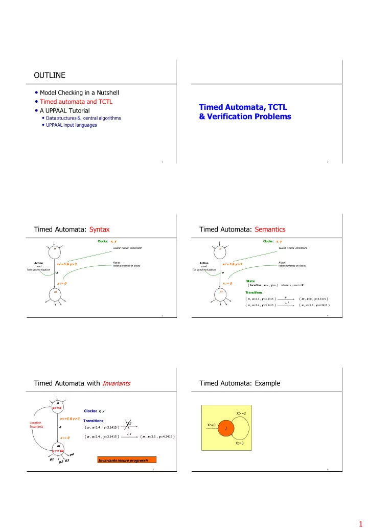
Timed Automata: Syntax
n m a Clocks: x, y x<=5 & y>3 x := 0
Guard =clock constraint Reset Action perfomed on clocks Action used for synchronization 4
Timed Automata: Semantics
n m a Clocks: x, y x<=5 & y>3 x := 0
Guard =clock constraint Reset Action perfomed on clocks
Transitions ( n , x=2.4 , y=3.1415 ) ( n , x=3.5 , y=4.2415 )
1.1
( n , x=2.4 , y=3.1415 ) ( m , x=0 , y=3.1415 )
a
State ( location , x=v , y=u )
where v,u are in R Action used for synchronization 5
n m a
Clocks: x, y
x<=5 & y>3 x := 0
Transitions ( n , x=2.4 , y=3.1415 ) ( n , x=3.5 , y=4.2415 )
1.1
( n , x=2.4 , y=3.1415 )
3.2 x<=5 y<=10 Location Invariants g1 g2 g3 g4
Invariants insure progress!!
Timed Automata with Invariants
6
Timed Automata: Example
l
X>=2 X:=0 X:=0