Outline Optimisation Discrete Introduction 1 Solving the Knapsack - - PowerPoint PPT Presentation

logoenac

Optimisation Discrete

Solving the Knapsack Problem Sonia Cafieri ENAC

sonia.cafieri@enac.fr

• S. Cafieri (ENAC)

Knapsack Problem 2016-2017 1 / 55 logoenac

Outline

1

Introduction

2

Heuristics for the Knapsack Problem

3

Solving the Continuous Knapsack Problem

4

Exact solution of the KP Branch and Bound algorithms for IP Branch and Bound for the KP Branch and Bound for IP : Remarks

• S. Cafieri (ENAC)

Knapsack Problem 2016-2017 2 / 55 logoenac

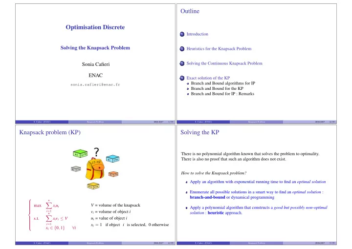
Knapsack problem (KP)

               max

n

• i=1

xiui s.t.

n

• i=1

xivi ≤ V xi ∈ {0, 1} ∀i V = volume of the knapsack vi = volume of object i ui = value of object i xi = 1 if object i is selected, 0 otherwise

• S. Cafieri (ENAC)

Knapsack Problem 2016-2017 4 / 55 logoenac

Solving the KP

There is no polynomial algorithm known that solves the problem to optimality. There is also no proof that such an algorithm does not exist. How to solve the Knapsack problem? Apply an algorithm with exponential running time to find an optimal solution Enumerate all possible solutions in a smart way to find an optimal solution : branch-and-bound or dynamical programming Apply a polynomial algorithm that constructs a good but possibly non-optimal solution : heuristic approach.

• S. Cafieri (ENAC)

Knapsack Problem 2016-2017 5 / 55

logoenac

Heuristics for KP : Greedy algorithm

Greedy : algorithm that makes the choice that looks the best at the moment. Idea : Sort by most rewarding items with respect to a given criterion and take as many of the top most valuable items as will fit.

Heuristic 1 :

sort ui i ∈ {1, . . . , n} by non-increasing order

Heuristic 2 :

sort vi i ∈ {1, . . . , n} by increasing order

Heuristic 3 :

sort ui/vi i ∈ {1, . . . , n} by non-increasing order ⇒ the most efficient greedy

• S. Cafieri (ENAC)

Knapsack Problem 2016-2017 7 / 55 logoenac

Greedy algorithm for KP

W ← 0 sort by most rewarding items for i = 1, . . . , n do W ← vi + W if (W ≤ V) then xi ← 1 else xi ← 0 W ← W − vi endif endfor

• S. Cafieri (ENAC)

Knapsack Problem 2016-2017 8 / 55 logoenac

0-1 Knapsack and Continuous Knapsack

0-1 Knapsack Problem: you can only choose to take all (1) or nothing (0) of a particular item Continuous Knapsack Problem (CNP): you can take any fractions of the items to put in the knapsack ⇒ continuous relaxation of 0-1 Knapsack For both versions : Optimal Substructure property: an optimal solution contains within it optimal solutions to subproblems.

If we remove item i from an optimal solution, then the remaining items must be optimal for the subproblem where the bag volume is V − vi and the available items do not include item i. Otherwise, we would be able to construct an even better solution than the optimal one.

• S. Cafieri (ENAC)

Knapsack Problem 2016-2017 10 / 55 logoenac

Solving the CKP

Greedy n.3

Idea : Sort by most rewarding items with respect to the ratio of value to size, and take as much as possible of the most valuable items as will fit. Steps :

1

compute ratios (densities) ui/vi

2

sort them by non-increasing order

3

take as much as possible of the densest item not already in the bag Complexity : O(n log n) for sorting, O(n) for greedy choices

• S. Cafieri (ENAC)

Knapsack Problem 2016-2017 11 / 55

logoenac

Solving the CKP

Greedy n.3

Sort values/volumes by non-increasing order. Let ij be the indexes of the objects after sorting (uij/vij with j = 1 is the maximum ratio): ui1 vi1 ≥ ui2 vi2 ≥ · · · ≥ uin vin W ← 0 for i ≤ n do if (W + vij ≤ V) then xij ← 1 /∗ take item i ∗/ W ← W + vij else xih ← V − W vih /∗ take a fraction of item i ∗/ xij ← 0 ∀j > h endif endfor

• S. Cafieri (ENAC)

Knapsack Problem 2016-2017 12 / 55 logoenac

Solving exactly the CKP

Theorem

The Greedy algorithm (n.3) is optimal for the Continuous Knapsack Problem (CKP) (continuous relaxation of 0-1 Knapsack)

• Proof. 1

Note that the algorithm fills the knapsack completely. It may take a fraction of an item, which can only be the last selected item. The greedy solution is such that there exists a h such that 1 = xi1 = xi2 = · · · = xih > xih+1 > xih+2 = · · · = xin = 0. We compare this solution with another (feasible) solution yi1, . . . , yin. Let k be the smallest index such that yik < 1, and let ℓ be the smallest index such that k < ℓ and yiℓ > 0. (such an ℓ exists, otherwise the y solution would be equal to the x solution).

• S. Cafieri (ENAC)

Knapsack Problem 2016-2017 13 / 55 logoenac

Solving exactly the CKP

• Proof. (cont.)

We increase yik and decrease yiℓ, while keeping all other values equal. Let ǫ = min{vik(1 − yik), viℓyiℓ}. We increase yik by ǫ vik and decrease yiℓ by ǫ viℓ , obtaining a new solution. This new solution is no worse than the y solution. Moreover, either yik has become 1, or yiℓ has become 0. Repeating the same argument we find the solution x of the greedy.

• S. Cafieri (ENAC)

Knapsack Problem 2016-2017 14 / 55 logoenac

Solving exactly the CKP

Theorem

The Greedy algorithm (n.3) is optimal for the Continuous Knapsack Problem (CKP) (continuous relaxation of 0-1 Knapsack)

• Proof. 2

Let O = {o1, o2, . . . , on} be the optimal solution and G = {g1, g2, . . . , gn} be the greedy solution (where the items are ordered with respect to the greedy choice). We show that there exist an optimal solution such that it also takes the greedy choice in each iteration. First, we show that an optimal solution selects (a fraction or 1 unit of) item g1.

• S. Cafieri (ENAC)

Knapsack Problem 2016-2017 15 / 55

logoenac

Solving exactly the CKP

• Proof. 2 (cont.)

Two cases:

1

G takes 1 unit of g1. If O also takes 1 unit of g1, done. If O doesn’t take 1 unit of g1, then we take away volume vg1 from O and put 1 unit of g1 to it ⇒ new solution O′. Of course O′ has the same volume constraint V as O. Moreover, g1 has maximum ratio u/v. ⇒ O′ is as good as O ⇒ g1 ∈ O′ and O′ is an optimal solution.

2

G takes a fraction f of g1 (the volume added to O is f × vg1). If O also takes a fraction f of g1, done. If O takes less than f of g1 (cannot take more because o optimal), then we take away f × vg1 from O and put f of g1 to it ⇒ new solution O′. As before, O′ is as good as O (otherwise contradiction).

• S. Cafieri (ENAC)

Knapsack Problem 2016-2017 16 / 55 logoenac

Solving exactly the CKP

• Proof. 2 (cont.)

Second, we observe that after each greedy choice is made, we have a problem of the same form as the original one. The problem exhibits the optimal substructure property ⇒ G ≡ O.

• S. Cafieri (ENAC)

Knapsack Problem 2016-2017 17 / 55 logoenac

Solving exactly the CKP

(Another) Alternative Proof: The simplex algorithm for solving the CKP takes exactly the same steps as the greedy. Let ih be such that : ∀ j ∈ {1, . . . , h} xij ← 1 ∀ j ∈ {h + 2, . . . , n} xij ← xih+1 ← V − h

j=1 vij

vih+1 that is, ih is such that:

h

• j=1

vij ≤ V and

h+1

• j=1

vij > V Let us apply the simplex algorithm with the dictionary representation.

• S. Cafieri (ENAC)

Knapsack Problem 2016-2017 18 / 55 logoenac

Solving exactly the CKP

(Another) Alternative Proof: (cont.)                      xn+1 = 1 − xi1 xn+2 = 1 − xi2 . . . x2n = 1 − xin x2n+1 = V − n

j=1 vijxij

z = n

j=1 uijxij

• S. Cafieri (ENAC)

Knapsack Problem 2016-2017 19 / 55

logoenac

Solving exactly the CKP

(Another) Alternative Proof: (cont.) pivot: xi1 ↔ xn+1                        xi1 = 1 − xn+1 xn+2 = 1 − xi2 . . . x2n = 1 − xin x2n+1 = V − n

j=2 vijxij − vi1(1 − xn+1) = (V − vi1) − n j=2 vijxij + vi1xn+1

z = ui1 + n

j=2 uijxij − ui1xn+1

We continue with following dictionaries.

• S. Cafieri (ENAC)

Knapsack Problem 2016-2017 20 / 55 logoenac

Solving exactly the CKP

(Another) Alternative Proof: (cont.) Dictionary h : pivot: xih ↔ xn+h                                  xi1 = 1 − xn+1 xi2 = 1 − xn+2 . . . xih = 1 − xn+h xn+h+1 = 1 − xih+1 x2n = 1 − xin x2n+1 = (V − h

j=1 vij) − n j=h+1 vijxij + h j=1 vijxn+j

z = h

j=1 uij + n j=h+1 uijxij − h j=1 ui1xn+j

• S. Cafieri (ENAC)

Knapsack Problem 2016-2017 21 / 55 logoenac

Solving exactly the CKP

(Another) Alternative Proof: (cont.) Dictionary h + 1 : pivot: xih+1 ↔ x2n+1                                      xi1 = 1 − xn+1 xi2 = 1 − xn+2 . . . xih = 1 − xn+h x2n = 1 − xin xih+1 = (V − h

j=1 vij)

vih+1 − n

j=h+2 vijxij

vih+1 + h

j=1 vijxn+j

vih+1 − x2n+1 vih+1 xn+h+1 = 1 − (expression of xih+1) z = h

j=1 uij + uih+1(expression of xih+1) + n j=h+2 uijxij − h j=1 uijxn+j

• S. Cafieri (ENAC)

Knapsack Problem 2016-2017 22 / 55 logoenac

Solving exactly the CKP

(Another) Alternative Proof: (cont.) Dictionary h + 1 : pivot: xih+1 ↔ x2n+1 z =

h

• j=1

uij + uih+1

• (V − h

j=1 vij)

vih+1

• +

n

• j=h+2
• uij − uih+1

vij vih+1

• xij

+

h

• j=1

vij vih+1 − uij

• xn+j

−x2n+1 vih+1

• S. Cafieri (ENAC)

Knapsack Problem 2016-2017 23 / 55

logoenac

Solving exactly the CKP

(Another) Alternative Proof: (cont.) We check the signs of the coefficients of the variables : ∀j = h + 2, . . . , n sign

• uij − uih+1

vij vih+1

• = sign

uij vij − uih+1 vih+1

• = −1

because j > h + 1 ∀j = 1, . . . , h sign uih+1 vih+1 vij − uij

• = sign

uih+1 vih+1 − uij vij

• = −1

because j < h + 1 Hence the simplex algorithm stops. ⇒ the (feasible) solution found is also the optimal solution.

• S. Cafieri (ENAC)

Knapsack Problem 2016-2017 24 / 55 logoenac

Solving the KP exactly

Can we solve the KP exactly? ⇓

Branch-and-Bound (B&B)

• S. Cafieri (ENAC)

Knapsack Problem 2016-2017 26 / 55 logoenac

Branch and Bound

Branch-and-Bound (B&B) is a general framework for solving exactly integer and discrete optimization problems. Intelligent implicit enumeration of all possible solutions

• nly potentially good solutions are enumerated,

solutions that cannnot lead to improve the current solution are not explored based on the observation that the enumeration of integer solutions has a tree structure.

• S. Cafieri (ENAC)

Knapsack Problem 2016-2017 28 / 55 logoenac

Branch and Bound - search tree

Search Tree : Nodes : represent stages of construction of the solution Arcs : represent choices made to build the solution

Exemple, for the KP: Nodes : represent a step in which some objects have been placed in the bag, some others have been left out of the bag, and for some others no decision has yet been taken. Arcs : indicate the action of putting an object in the bag or not putting it in the bag

• S. Cafieri (ENAC)

Knapsack Problem 2016-2017 29 / 55

logoenac

Branch and Bound - idea

The nodes of the search tree represent subsets of all of the possible solutions. In particular, the root node represents all solutions that can be generated by growing the tree. The main idea is to build step by step the search tree avoiding growing the whole tree as much as possible. Only the most promising nodes are generated and explored at any stage. The node that is the most promising is determined by estimating a bound on the best value of the objective function that can be obtained by growing that node to later stages.

• S. Cafieri (ENAC)

Knapsack Problem 2016-2017 30 / 55 logoenac

Branch and Bound - main steps

Branching : a node is selected for further growth and two new subproblems are created Bounding : upper and lower bounds on the best value attained by growing a node are estimated Pruning : nodes that are showed to be never either feasible or optimal are permanently discarded

• S. Cafieri (ENAC)

Knapsack Problem 2016-2017 31 / 55 logoenac

Branch and Bound - main steps

During the search, a node must be in one of the following states : (i) has no feasible solution (ii) is such that its associated solution xS is feasible and

(a) xS has a value better than the incumbent * (b) xS has a value no better than the incumbent *

(iii) neither of states (i) and (ii) has yet been established. A node in either state (i) or (ii) is said to be fathomed. A node that has not yet been fathomed is said to be active. A node in states (i) or (iib) cannot contain the optimum, it is pruned from the tree. * incumbent = best integer solution found so far

• S. Cafieri (ENAC)

Knapsack Problem 2016-2017 32 / 55 logoenac

Branch and Bound - main steps

The search continues, branching from the active nodes until either : (i) all nodes have been pruned from the tree (in which case the problem has no feasible solutions) (ii) all active nodes have bounds no greater than the value of the incumbent (in which case the incumbent represents an optimal solution)

• S. Cafieri (ENAC)

Knapsack Problem 2016-2017 33 / 55

logoenac

Branch and Bound for KP - principles

The solution set is partitioned into subsets S1, . . . , SM each subset corresponds to a partial (feasible) solution,

i.e. some of the variables have been fixed

When a branching with respect to a variable xj is done, 2 new subsets are created from Sk : S0

k where we set xj = 0,

S1

k where we set xj = 1

An upper bound UBk corresponding to Sk can be computed by the greedy algorithm on the CKP corresponding to Sk

(integer part)

A lower bound LBk corresponding to Sk can be computed by rounding down the fractional variable, if it exists. If UBk = LBk the subproblem k is solved exactly.

• S. Cafieri (ENAC)

Knapsack Problem 2016-2017 35 / 55 logoenac

Branch and Bound for KP - principles

When we continue branching ? Let z∗ be the value of the best feasible solution found so far: current best solution: z∗ ≥ max{LBk, ∀k} UBk > z∗ : the subset Sk may contain a feasible solution with value > z∗. We continue working on Sk. (Sk, UBk) is active ⇒ Branching UBk ≤ z∗ : the subset Sk cannot contain a solution with value > z∗. The subset is of no interest anymore. ⇒ Fathoming

• S. Cafieri (ENAC)

Knapsack Problem 2016-2017 36 / 55 logoenac

Branch and Bound for KP - steps

Initialization construct a list L containing all active pairs (Sk, UBk) : initially, the original problem initial Upper Bound UB : solution of the CKP via the greedy algorithm initial Lower Bound LB : a feasible solution (rounding down the value of the fractional variable in the solution of CKP)

• S. Cafieri (ENAC)

Knapsack Problem 2016-2017 37 / 55 logoenac

Branch and Bound for KP - steps

As long as L is not empty : choose among the active pairs the one with the maximal UB : (Sk, UBk) split Sk in S0

k and S1 k according to a branching criterion

(ex. : the fractional variable xi in the continuous solution)

compute UB0

k and UB1 k (greedy algorithm for CNP)

compute LB0

k and LB1 k (feasible solution for KP)

if LB0

k > z∗, then set z∗ ← LB0 k

and update x∗ accordingly if LB1

k > z∗, then set z∗ ← LB1 k

and update x∗ accordingly if UB0

k > z∗, then add (S0 k, UB0 k) to L

if UB1

k > z∗, then add (S1 k, UB1 k) to L

update L deleting the elements (Sh, UBh) such that UBh < z∗

• S. Cafieri (ENAC)

Knapsack Problem 2016-2017 38 / 55

logoenac

Branch and Bound for KP - algorithm

Sort values/volumes by non-increasing order. Let ij be indexes such that uij/vij with j = 1 is the maximum ratio xi ← 2 ∀i k ← 1

// iteration counter

L ← (Sk, UBk)

// original problem

z∗ ← LBk while (L not empty) do ν ← min{ij|j ∈ {1, ..n} ∧ xν = 2} x0

ν ← 0,

x1

ν ← 1

// two branches

for p = 0, 1 do compute UBp

k

and LBp

k

if (UBp

k > z∗

and LBp

k = UBp k) then

add (Sp

k, UBp k) to L by non-increasing order for UB

• S. Cafieri (ENAC)

Knapsack Problem 2016-2017 39 / 55 logoenac

Branch and Bound for KP - algorithm (cont.)

if (LBp

k > z∗) then

z∗ ← LBp

k

// current best solution

x∗ ← corresponding solution end if end for L ← L \ (Sk, UBk) k ← k + 1 end while

• S. Cafieri (ENAC)

Knapsack Problem 2016-2017 40 / 55 logoenac

Example

     max z = 12x1 + 11x2 + 8x3 + 6x4 s.t. 8x1 + 8x2 + 6x3 + 5x4 ≤ 20 xi ∈ {0, 1} ∀i u1 v1 > u2 v2 > u3 v3 > u4 v4

• S. Cafieri (ENAC)

Knapsack Problem 2016-2017 41 / 55 logoenac

Designing a Branch and Bound algorithm

Branch and Bound is a very general framework. To completely specify how the process is to proceed, you also need to define How to obtain bounds? How to branch (partition into subproblems)? In what order to branch on variables? In what order to examine nodes?

• S. Cafieri (ENAC)

Knapsack Problem 2016-2017 43 / 55

logoenac

Branch and Bound: Obtaining bounds

For a maximization problem

• the (current) tightest lower bound, provided by the best solution we have found,

is also referred to as the primal bound.

• the upper bound on the profit obtainable within a given set of solutions

is also referred to as the dual bound.

To obtain a dual (upper) bound :

• ne typically solves a relaxation of the subproblem :

LP (continuous) relaxation (but also Lagrangian relaxation, etc..) The bound can also be computed by solving the dual problem. To obtain a primal (lower) bound :

• ne typically computes a feasible solution of the subproblem.
• S. Cafieri (ENAC)

Knapsack Problem 2016-2017 44 / 55 logoenac

Dual Problem

For a LP problem in standard Primal form: (LP)        max cTx x ∈ Rn, c ∈ Rn s.t. Ax ≤ b A ∈ Rm×n, b ∈ Rm x ≥ 0 The Dual Problem is : (D)        min bTy y ∈ Rm s.t. ATy ≥ c y ≥ 0

• S. Cafieri (ENAC)

Knapsack Problem 2016-2017 45 / 55 logoenac

Dual Problem

To obtain the Dual Problem:

• write the Lagrangian :

L(x, y, s) = cTx − sTx + yT(b − Ax), with s ∈ Rn, y ∈ Rm (using nonnegative Lagrangian multipliers to add the constraints to the objective function)

• write the Lagrangian dual :

min max(yb + (cT − s − yA)x)

• apply the optimality conditions (KKT) to the Lagrangian dual

The solution of the dual problem provides an upper bound to the solution of the primal problem

• S. Cafieri (ENAC)

Knapsack Problem 2016-2017 46 / 55 logoenac

Dual Problem : Example

Knapsack with 2 constraints, relaxed

                             max

n

• i=1

xiui s.t.

n

• i=1

xivi ≤ V

n

• i=1

xipi ≤ P xi ≤ 1 ∀i xi ≥ 0 ∀i A =        v1 . . . vn p1 . . . pn 1 . . . . . . . . . . . . 1        b =        V P 1 . . . 1       

• S. Cafieri (ENAC)

Knapsack Problem 2016-2017 47 / 55

logoenac

Dual Problem : Example

Knapsack with 2 constraints, relaxed

AT =    v1 p1 1 . . . . . . . . . . . . vn pn . . . 1    (D)            min bTy =

n+2

• i=1

biyi s.t. ATy ≥ u ⇔ viy1 + piy2 + yi+2 ≥ ui ∀i ∈ {1, ..n} y ≥ 0

• S. Cafieri (ENAC)

Knapsack Problem 2016-2017 48 / 55 logoenac

Dual Problem : Example

Knapsack with 2 constraints, relaxed

A (feasible) solution can be obtained by setting : y1 = y2 = 0, yi+2 = ui ∀i The solution is :

n

• i=1

ui. This gives an upper bound for the 0-1 KP. Another solution can be obtained by setting : y1 = y2 = 1, yi+2 = max{0, ui − pi − vi ∀i} The solution is : V + P +

n

• i=1

max{0, ui − pi − vi} that can be better than the previous one if V + P <

n

• i=1

ui. So, we can search for min

α∈R+ α(V + P) + max{0, ui − α(pi + vi)}

• S. Cafieri (ENAC)

Knapsack Problem 2016-2017 49 / 55 logoenac

Branch and Bound: How to partition into subproblems

IP problems

• choose xj /

∈ Z

• set

Sj

k = Sk ∪ {x : xj ≤ ⌊xk j ⌋}

and Sj+1

k

= Sk ∪ {x : xj ≤ ⌊xk

j ⌋ + 1}

How to choose the fractionary component? Example : choose the component with fractionary value closest to 0.5

Binary IP problems

• choose xj
• set S0

k = Sk ∪ {x : xj = 0}

and S1

k = Sk ∪ {x : xj = 1}

• S. Cafieri (ENAC)

Knapsack Problem 2016-2017 50 / 55 logoenac

Branch and Bound: In what order of variables to branch?

Recall the previous example:      max z = 12x1 + 11x2 + 8x3 + 6x4 s.t. 8x1 + 8x2 + 6x3 + 5x4 ≤ 20 xi ∈ {0, 1} ∀i

• S. Cafieri (ENAC)

Knapsack Problem 2016-2017 51 / 55

logoenac

branching on the variable with lowest index

• S. Cafieri (ENAC)

Knapsack Problem 2016-2017 52 / 55 logoenac

branching on fractional variables

• S. Cafieri (ENAC)

Knapsack Problem 2016-2017 53 / 55 logoenac

Branch and Bound: How to choose a node

The search tree can be explored using Depth-first search allows to find a feasible solution to the IP quickly Breadth-first-search may allow to prune more of the search tree sooner Best-Node First chooses the node with the best dual bound. This might lead to finding a good incumbent quickly, thus eliminating the need to evaluate the other subproblems Other heuristics

• S. Cafieri (ENAC)

Knapsack Problem 2016-2017 54 / 55 logoenac

Bibliography I

L.R. Foulds. Combinatorial Optimization for Undergraduates Springer-Verlag, 1984. C.H. Papadimitriou and K. Steiglitz. Combinatorial Optimization: Algorithms and Complexity. Dover, New York, 1998. John W. Chinneck. Practical Optimization: a gentle introduction www.sce.carleton.ca/faculty/chinneck/po.html, 2010.

• S. Cafieri (ENAC)

Knapsack Problem 2016-2017 55 / 55