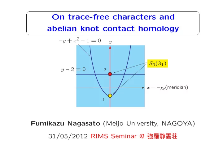
On trace-free characters and abelian knot contact homology y + - PowerPoint PPT Presentation

✓ ✏ On trace-free characters and abelian knot contact homology ✒ ✑ − y + x 2 − 1 = 0 y S 0 (3 1 ) y − 2 = 0 2 x = − χ ρ (meridian) -1 Fumikazu Nagasato (Meijo University, NAGOYA) 31/05/2012 RIMS Seminar @ 強羅静雲荘

Notations K : a knot in S 3 E K := S 3 − N ( K ) G ( K ) := π 1 ( E K ), knot group R ( K ) := { ρ : G ( K ) → SL 2 ( C ) , representation } X ( K ) := { χ ρ : G ( K ) → C , characters of ρ ∈ R ( K ) } � � S 0 ( K ) := X ( K ) ∩ χ ρ ( meridian ) = 0 trace-free characters HC ab 0 ( K ) : degree 0 abelian knot contact homology of K introduced by Lenhard Ng � [Ng] Knot and braid invariants from contact homology � I and II , Geom. Topol. 9 (2005) 1

Main theorem Let G ( K ) = � m 1 , · · · , m n | r 1 = 1 , · · · , r n = 1 � be a Wirtinger presentation. Then S 0 ( K ) is realized as the algebraic set ⎧ � ⎫ � (1) x ka = x ij x ia − x ja , x kab = x ij x iab − x jab ⎪ ⎪ ⎪ � ⎪ ⎪ ⎪ ⎪ � ⎛ ⎞ ⎪ ⎪ ⎪ ⎪ � ⎪ ⎪ ⎪ ⎪ � ⎪ ⎪ ⎪ ∀ Wirtinger triple ⎜ k ⎟ ⎪ � ⎪ ⎪ ⎪ ⎜ ⎟ ⎪ � ⎪ ⎝ a, b ∈ { 1 , · · · , n } , ⎪ ⎪ ⎪ � ⎠ ⎪ ⎪ ⎪ i j ⎪ � ( i, j, k ) ⎪ ⎪ ⎪ ⎪ � ⎪ ⎪ ⎪ ⎪ � ⎪ ⎪ ⎪ ⎪ � ⎪ � � ⎪ ⎪ ⎪ � ⎪ ( x ab ; x pqr ) ∈ C ( n 2 ) + ( n � � ⎪ ⎪ 3 ) x i 1 j 1 x i 1 j 2 x i 1 j 3 ⎪ � ⎪ � � ⎪ ⎪ ⎪ � ⎪ � � ⎨ ⎬ (2) x i 1 i 2 i 3 · x j 1 j 2 j 3 = 1 � x i 2 j 1 x i 2 j 2 x i 2 j 3 � � � 2 � � (1 ≤ a < b ≤ n ) � � � ⎪ x i 3 j 1 x i 3 j 2 x i 3 j 3 ⎪ ⎪ � ⎪ ⎪ ⎪ ⎪ � ⎪ ⎪ ⎪ ⎪ � ⎪ (1 ≤ p < q < r ≤ n ) ⎪ ⎪ (1 ≤ i 1 < i 2 < i 3 ≤ n , 1 ≤ j 1 < j 2 < j 3 ≤ n ) ⎪ � ⎪ ⎪ ⎪ ⎪ � ⎪ ⎪ ⎪ ⎪ � ⎪ ⎪ � � ⎪ ⎪ ⎪ � � � ⎪ ⎪ 2 x 12 x 1 a x 1 b ⎪ � ⎪ ⎪ � � ⎪ ⎪ � ⎪ ⎪ � � ⎪ ⎪ � ⎪ x 21 2 x 2 a x 2 b � � ⎪ ⎪ ⎪ � ⎪ (3) = 0 � � ⎪ (3 ≤ a < b ≤ n ) ⎪ ⎪ � ⎪ x a 1 x a 2 2 x ab ⎪ � � ⎪ ⎪ � ⎪ � � ⎪ ⎪ ⎪ � ⎪ � � ⎩ ⎭ x b 1 x b 2 x ba 2 � 2

(1) x ka = x ij x ia − x ja (F2) , x kab = x ij x iab − x jab (F3) the fundamental relations (F) � � � � x i 1 j 1 x i 1 j 2 x i 1 j 3 � � � � (2) x i 1 i 2 i 3 · x j 1 j 2 j 3 = 1 x i 2 j 1 x i 2 j 2 x i 2 j 3 � � 2 � � � � x i 3 j 1 x i 3 j 2 x i 3 j 3 the hexagon relations (H) � � � � 2 x 12 x 1 a x 1 b � � � � x 21 2 x 2 a x 2 b � � (3) = 0 � � � x a 1 x a 2 2 x ab � � � � � x b 1 x b 2 x ba 2 the rectangle relations (R) NOTE. x aa := 2, x ba := x ab (symmetric) x i σ (1) i σ (2) i σ (3) := sign( σ ) x i 1 i 2 i 3 ( σ ∈ S 3 ) (anti-sym) x aab = 0 3

Plan of this talk Section 1: An observation of the main theorem Section 2: A rought sketch of proof of the main theorem Section 3: An application to abelian knot contact homology (Ng’s conjecture on abelian knot contact homology)

Section 1: An observation of the main theorem How to get the fundamental relations (F)

Realizing X ( K ) as an algebraic set (a short review) x = m 1 � y = m 1 m − 1 � 2 ✓ ✏ x := − tr( ρ ( � x )) = − tr( m 1 ) K m = m 1 y )) = − tr( m 1 m − 1 y := − tr( ρ ( � 2 ) m 2 ... ✒ ✑ ✓ ✏ Theorem [Gelca-N (JKTR) ], [N (Bull. Korean Math.) ] ( x, y ) ∈ C 2 � � � � X ( K m ) = � ( y − 2) R m ( x, − y ) = 0 , where R m ( x, y ) := S m ( y ) − S m − 1 ( y ) + x 2 � m − 1 i =0 S i ( y ) S n +2 ( z ) = zS n +1 ( z ) − S n ( z ) , S 1 ( z ) = z, S 0 ( z ) = 1 . ✒ ✑ − y + x 2 − 1 EX. R 1 ( x, − y ) = y 2 − x 2 y + y + x 2 − 1 R 2 ( x, − y ) = 4

Realizing S 0 ( K ) as an algebraic set (a short review) ( x, y ) ∈ C 2 � � � � � � − y + x 2 − 1 X (3 1 ) = � ( y − 2) = 0 − y + x 2 − 1 = 0 y = − tr( ρ ( m 1 m − 1 − y + x 2 − 1 = 0 2 )) y = − tr( ρ ( m 1 m − 1 2 )) S 0 (3 1 ) y − 2 = 0 y − 2 = 0 2 2 x = − tr( ρ ( m 1 )) x = − tr( ρ ( m 1 )) − 1 − 1 X (3 1 ) ⊂ C 2 S 0 (3 1 ) = X (3 1 ) ∩ { tr( ρ ( m 1 )) = 0 } ✓ ✏ Definition ( S 0 ( K ) as an algebraic set) S 0 ( K ) := X ( K ) ∩ { tr( ρ ( µ )) = 0 } (w/o multiplicity) ✒ ✑ We want to calculate S 0 ( K ) directly w/o the calculation of X ( K ). 5

Realizing S 0 ( K ) as an algebraic set (a short review) ( x, y ) ∈ C 2 � � � y 2 + y − 1 − x 2 y + x 2 � � � X (4 1 ) = � ( y − 2) = 0 y 2 + y − 1 − x 2 y + x 2 = 0 y = − tr( ρ ( m 1 m − 1 2 )) y − 2 = 0 2 x = − tr( ρ ( m 1 )) √ � � 2 , − 1 ± 5 S 0 (4 1 ) = X (4 1 ) ∩ { tr( ρ ( m 1 )) = 0 } = 2 This can be done because we have the defining poly. of X ( K m ). We want to calculate S 0 ( K ) directly w/o the calculation of X ( K ). 6

A decomposition of E K into H n and handles 2 ∪ ∪ = 4 ∪ xxxxxxxxxxxxxxxx xxxxxxxxxxxxxxxx xxxxxxxxxxxxxxxx xxxxxxxxxxxxxxxx xxxxxxxxxxxxxxxx 1 3 ∪ ∪ 3-handle 2-handles E 4 1 H 4 2 1 2 3 4 1 3 4 7

Presenting attaching curves on a punctured disk 3 2 1 2 3 4 push inside 4 1 draw the "cores" 3 2 2 3 turn 4 upside down 4 4 1 1 8

✓ ✏ ⎧ ⎪ x 13 x 23 − x 12 = 2 , x 13 = x 23 ⎪ ⎪ ⎪ 3 2 ⎪ ⎪ ⎪ x 12 x 24 − x 14 = 2, x 12 = x 24 ⎪ ⎪ ⎨ x 13 x 14 − x 34 = 2, x 13 = x 14 ⎪ ⎪ ⎪ ⎪ ⎪ x 24 x 34 − x 23 = 2, x 23 = x 24 ⎪ ⎪ 4 ⎪ 1 ⎪ ⎩ a part of (F2) ✒ ✑ EX. For an arbitrary trace-free character χ ρ : � � 1 = m 3 m 1 m − 1 3 m − 1 ρ ( m 3 m 1 m − 1 3 m − 1 − 2 = − tr 2 ) 2 3 3 2 3 2 2 = = − − 4 4 1 4 1 1 � � � � � � ρ ( m 3 m 1 m − 1 ρ ( m − 1 ρ ( m 3 m 1 m − 1 − 2 = − tr 3 ) tr 2 ) + tr 3 m 2 ) 9

✓ trace-free Kauffman brakcet skein relation (at t = − 1 ) ✏ = − − = 0 = − 2 , , ✒ ✑ 3 3 2 2 = = − 1 4 1 4 � � − 2 = − tr( ρ ( m 3 m 1 m − 1 3 m − 1 ρ ( m 3 m 1 m − 1 2 )) = tr 3 m 2 ) ✓ ✏ in general a loop γ in E K ⇔ − t [ γ ] ( ρ ) := − tr( ρ ([ γ ])) ( χ ρ ∈ S 0 ( K )) trace-free KBSR ⇔ trace-identity ✒ ✑ 10

✓ trace-free Kauffman brakcet skein relation (at t = − 1 ) ✏ = − − = − 2 = 0 , , ✒ ✑ 2 3 2 3 = = − 4 4 1 1 � � − 2 = − tr( ρ ( m 3 m 1 m − 1 3 m − 1 ρ ( m 3 m 1 m − 1 2 )) = tr 3 m 2 ) Here, by skein relation, we obtain ✓ ✏ + + = ✒ ✑ 10-a

✓ trace-free Kauffman brakcet skein relation (at t = − 1 ) ✏ = − − = − 2 = 0 , , ✒ ✑ 3 3 2 2 = = − 1 4 1 4 � � − 2 = − tr( ρ ( m 3 m 1 m − 1 3 m − 1 ρ ( m 3 m 1 m − 1 2 )) = tr 3 m 2 ) 3 3 2 2 = − + 4 1 4 1 � � � � ρ ( m 2 m − 1 3 m − 1 ρ ( m 1 m 2 = tr ( ρ ( m 1 m 3 )) tr 3 ) + tr 2 ) · · · continued 10-b

� � ρ ( m 2 m − 1 + tr( ρ ( m − 1 2 m 1 m 2 − 2 = · · · = tr( ρ ( m 1 m 3 ))tr 3 ) 3 )) = tr ( ρ ( m 1 m 3 )) { tr( ρ ( m 2 ))tr( ρ ( m 3 )) − tr ( ρ ( m 2 m 3 )) } � � +tr( ρ ( m − 1 ρ ( m − 1 2 m 1 m 3 ))tr( ρ ( m 3 )) − tr 2 m 1 ) = − tr( ρ ( m 1 m 3 ))tr( ρ ( m 2 m 3 )) + tr( ρ ( m 1 m 2 )) 2 3 2 3 = · · · = − + 4 1 4 1 Set the followings: j j k i x i := = 0 , x ij := , x ijk := i i − tr( ρ ( m i )) = 0 − tr( ρ ( m i m j )) − tr( ρ ( m 1 m j m k )) − 2 = − x 13 x 23 + x 12 (the desired equation) 11

Also we can get: x 13 = x 23 , x 12 = x 24 , x 13 = x 14 , x 23 = x 24 EX. 2 3 3 2 x 13 = sl b ( x 13 ) := = = x 23 1 4 4 1 b x 12 = x 2 13 − 2 , x 24 = x 2 13 − 2, x 34 = x 2 Other relations: 13 − 2 EX. b 3 2 2 3 2 3 x 12 = sl b ( x 12 ) = = = 1 4 1 4 1 4 = − − 1 3 1 3 1 3 = x 2 13 − 2 12

Continuing this work, we obtain all the (F2): ⎧ ⎫ x 13 x 23 − x 12 = 2, x 12 x 24 − x 14 = 2, x 13 x 14 − x 34 = 2, x 24 x 34 − x 23 = 2 ⎪ ⎪ ⎪ ⎪ ⎪ ⎪ ⎪ ⎪ ⎪ ⎪ ⎪ ⎪ ⎪ x 13 = x 23 , x 12 = x 24 , x 13 = x 14 , x 23 = x 24 ⎪ ⎪ ⎪ ⎪ ⎪ ⎨ ⎬ x 12 = x 2 13 − 2 , x 24 = x 2 13 − 2, x 34 = x 2 13 − 2 ⎪ ⎪ ⎪ ⎪ ⎪ ⎪ ⎪ ⎪ x 13 = x 14 x 24 − x 12 , x 14 = x 23 x 34 − x 24 ⎪ ⎪ ⎪ ⎪ ⎪ ⎪ ⎪ ⎪ ⎪ ⎪ ⎩ ⎭ x 13 = x 23 x 24 − x 34 , x 23 = x 12 x 14 − x 24 ⎧ � ⎫ � ⎪ ⎪ x ka = x ik x ia − x ja (F2) ⎪ � ⎪ ⎪ ⎪ ⎨ � ⎬ � ( x 12 , · · · , x 45 ) ∈ C 10 F 2 (4 1 ) := � for any Wirtinger triple ( i, j, k ) ⎪ � ⎪ ⎪ ⎪ ⎪ � ⎪ ⎩ ⎭ � a ∈ { 1 , · · · , 4 } ( x aa = 2) So F 2 (4 1 ) is parametrized by x 13 and x 13 = x 13 ( x 2 13 − 2) − ( x 2 x 13 = x 14 x 24 − x 12 13 − 2) ( x 13 − 2)( x 2 13 + x 13 − 1) = 0 � � √ 2 , − 1 ± 5 Hence we get F 2 (4 1 ) = = S 0 (4 1 ) . 2 13

✓ ✏ ⎧ 3 2 x 123 = 0, x 124 = 0 ⎪ ⎪ ⎨ x 134 = 0, x 234 = 0 ⎪ ⎪ ⎩ (F3) becomes trivial ! 1 4 ✒ ✑ Indeed, we can check this like... b EX. j k j k x ijk = sl b ( x ijk ) = = i i j k = = − x i x ij − x i = 0 i 14