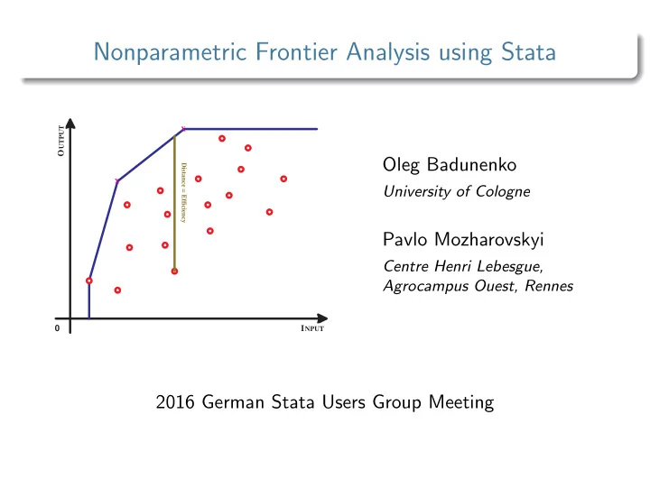
Nonparametric Frontier Analysis using Stata UTPUT X O Oleg - PowerPoint PPT Presentation

Nonparametric Frontier Analysis using Stata UTPUT� X� O� Oleg Badunenko Distance = Efficiency� X� University of Cologne Pavlo Mozharovskyi Centre Henri Lebesgue, Agrocampus Ouest, Rennes 0� I� NPUT� 2016 German Stata Users Group Meeting

Overview 1. Nonparametric frontier analysis Motivation Radial efficiency analysis Nonradial efficiency analysis 2. Statistical inference in radial frontier model Type of the bootstrap for statistical inference Returns to scale and scale analysis 3. Stata commands tenonradial , teradial , teradialbc , nptestind , and nptestrts 4. Empirical application Data: CCR81 Data: PWT5.6 5. Discussion Sample restriction and runtime Comparison to dea command in Stata, Stata Journal, 10(2): 267-80 Concluding remarks

Outline 1. Nonparametric frontier analysis Motivation Radial efficiency analysis Nonradial efficiency analysis 2. Statistical inference in radial frontier model Type of the bootstrap for statistical inference Returns to scale and scale analysis 3. Stata commands tenonradial , teradial , teradialbc , nptestind , and nptestrts 4. Empirical application Data: CCR81 Data: PWT5.6 5. Discussion Sample restriction and runtime Comparison to dea command in Stata, Stata Journal, 10(2): 267-80 Concluding remarks

Nonparametric frontier analysis Motivation Technical efficiency measurement UTPUT� X� O� Distance = Efficiency� X� 0� I� NPUT� Oleg Badunenko & Pavlo Mozharovskyi Nonparametric Efficiency Using Stata Stata Meeting 2016 4 / 48

Nonparametric frontier analysis Radial efficiency analysis Radial efficiency analysis ⊡ We assume that under technology T the data ( y , x ) are such that outputs are producible by inputs T = { ( x , y ) : y are producible by x } . (1) ⊡ The technology is fully characterized by its production possibility set, P ( x ) ≡ { y : ( x , y ) ∈ T } (2) or input requirement set, L ( y ) ≡ { x : ( x , y ) ∈ T } . (3) ⊡ Conditions (2) and (3) imply that the available outputs and inputs are feasible. Oleg Badunenko & Pavlo Mozharovskyi Nonparametric Efficiency Using Stata Stata Meeting 2016 5 / 48

Nonparametric frontier analysis Radial efficiency analysis Radial efficiency analysis (cont.) ⊡ The upper boundary of the production possibility set and lower boundary of the input requirement set define the frontier. ⊡ How far a given data point is from the frontier represents its efficiency. ⊡ In output-based radial efficiency measurement, the amount of necessary (proportional) expansion of outputs to move a data point to a boundary of the production possibility set P ( x ) serves a measure of technical efficiency. ⊡ In input-based radial efficiency measurement, it is the amount of necessary (proportional) reduction of inputs to move a data point to a boundary of the input requirement set L ( y ). Oleg Badunenko & Pavlo Mozharovskyi Nonparametric Efficiency Using Stata Stata Meeting 2016 6 / 48

Nonparametric frontier analysis Radial efficiency analysis Radial efficiency analysis (cont.) ⊡ Hypothetical one-input one-output production processes with three different technologies CRS, VRS and NIRS Output Output ✻ ✻ CRS CRS s s NIRS NIRS s s s ( x j , y j ) s ( x j , y j ) s s s ( x i , y i ) s s s ( x i , y i ) VRS VRS ✲ ✲ Input Input Figure: Output-based Figure: Input-based Oleg Badunenko & Pavlo Mozharovskyi Nonparametric Efficiency Using Stata Stata Meeting 2016 7 / 48

Nonparametric frontier analysis Radial efficiency analysis Radial efficiency analysis (cont.) ⊡ Empirically, an estimate of the radial Debreu-Farrell output-based measure of technical efficiency can be calculated by solving a linear programming problem for each data point k ( k = 1 , . . . , K ): ˆ F o k ( y k , x k , y , x | CRS) = max θ, z θ � K s.t. z k y km ≥ y km θ m , m = 1 , · · · , M , k =1 K � z k x kn ≤ x kn , n = 1 , · · · , N , k =1 z k ≥ 0 . y is K × M matrix of available data on outputs, x is K × N matrix of available data on inputs. Oleg Badunenko & Pavlo Mozharovskyi Nonparametric Efficiency Using Stata Stata Meeting 2016 8 / 48

Nonparametric frontier analysis Radial efficiency analysis Radial efficiency analysis (cont.) ⊡ This specifies constant returns to scale technology (CRS). � K ⊡ For variable returns to scale (VRS) a convexity constraint z k = 1 k =1 is added, while � K ⊡ for non-increasing returns to scale (NIRS), z k ≤ 1 inequality is k =1 added. Oleg Badunenko & Pavlo Mozharovskyi Nonparametric Efficiency Using Stata Stata Meeting 2016 9 / 48

Nonparametric frontier analysis Nonradial efficiency analysis Nonradial efficiency analysis ⊡ For data point ( y k , x k ), radial measure expands (shrinks) all M outputs y k = ( y k 1 , . . . , y kM ) ( N inputs x k = ( x k 1 , . . . , x kN )) proportionally until the frontier is reached. ⊡ At the reached frontier point, some but not all outputs (inputs) can be expanded (shrunk) while remaining feasible. ⊡ Nonradial measure of technical efficiency, the Russell measure. Oleg Badunenko & Pavlo Mozharovskyi Nonparametric Efficiency Using Stata Stata Meeting 2016 10 / 48

Nonparametric frontier analysis Nonradial efficiency analysis Nonradial efficiency analysis (cont.) ⊡ Output based, RM o k ( y k , x k , y , x | CRS)   � M   M − 1 θ m : ( θ 1 y k 1 , . . . θ M y kM ) ∈ P ( x ) , = max  . (4) m =1  θ m ≥ 0 , m = 1 , . . . , M ⊡ The input-based counterpart is given by RM i k ( y k , x k , y , x | CRS)   � N   N − 1 λ n : ( λ 1 x k 1 , . . . λ N y kN ) ∈ L ( y ) , = min  . (5) n =1  λ n ≥ 0 , n = 1 , . . . , N Oleg Badunenko & Pavlo Mozharovskyi Nonparametric Efficiency Using Stata Stata Meeting 2016 11 / 48

Nonparametric frontier analysis Nonradial efficiency analysis Nonradial efficiency analysis (cont.) ⊡ Since the Russell measure can expand (shrink) an output (input) vector at most (least) as far as the radial measure can, we have the result that o 1 ≥ � k ( y k , x k , y , x | CRS) ≥ ˆ F o RM k ( y k , x k , y , x | CRS) (6) and i 0 < � k ( y k , x k , y , x | CRS) ≤ ˆ F i RM k ( y k , x k , y , x | CRS) ≤ 1 . (7) Oleg Badunenko & Pavlo Mozharovskyi Nonparametric Efficiency Using Stata Stata Meeting 2016 12 / 48

Outline 1. Nonparametric frontier analysis Motivation Radial efficiency analysis Nonradial efficiency analysis 2. Statistical inference in radial frontier model Type of the bootstrap for statistical inference Returns to scale and scale analysis 3. Stata commands tenonradial , teradial , teradialbc , nptestind , and nptestrts 4. Empirical application Data: CCR81 Data: PWT5.6 5. Discussion Sample restriction and runtime Comparison to dea command in Stata, Stata Journal, 10(2): 267-80 Concluding remarks

Statistical inference in radial frontier model Type of the bootstrap for statistical inference Statistical inference ⊡ The estimated technical efficiency measures are too optimistic , due to the fact that UTPUT� X� the DEA estimate of the O� Distance = Efficiency� production set is necessarily a X� weak subset of the true production set under standard assumptions underlying DEA. ⊡ The statistical inference regarding the radial DEA 0� I� NPUT� estimates can be provided via bootstrap technique. Oleg Badunenko & Pavlo Mozharovskyi Nonparametric Efficiency Using Stata Stata Meeting 2016 14 / 48

Statistical inference in radial frontier model Type of the bootstrap for statistical inference Type of the bootstrap for statistical inference ⊡ The major assumption of the bootstrapping technique depends on whether the estimated output-based measures of technical efficiency are independent of the mix of outputs. ⊡ This dependency is testable given the assumption of returns to scale of the global technology ( nptestind command). ⊡ If output-based measures of technical efficiency are independent of the mix of outputs, the smoothed homogeneous bootstrap can be used. ⊡ This type of the bootstrap is not computer intensive. ⊡ Otherwise, the heterogenous bootstrap must be used to provide valid statistical inference. ⊡ The latter type of bootstrap is quite computer demanding and may take a while for large data sets. ⊡ Both implemented in teradialbc . Oleg Badunenko & Pavlo Mozharovskyi Nonparametric Efficiency Using Stata Stata Meeting 2016 15 / 48

Statistical inference in radial frontier model Returns to scale and scale analysis Technology and scale analysis ⊡ The assumption regarding the global technology is crucial in DEA. ⊡ The assumption about returns to scale should be made using prior knowledge about the particular industry. ⊡ If this knowledge does not suffice, or is not conclusive, the returns to scale assumption can be tested econometrically. ⊡ Moreover, if technology is not CRS globally, estimating measure of technical efficiency under CRS will lead to inconsistent results. Oleg Badunenko & Pavlo Mozharovskyi Nonparametric Efficiency Using Stata Stata Meeting 2016 16 / 48