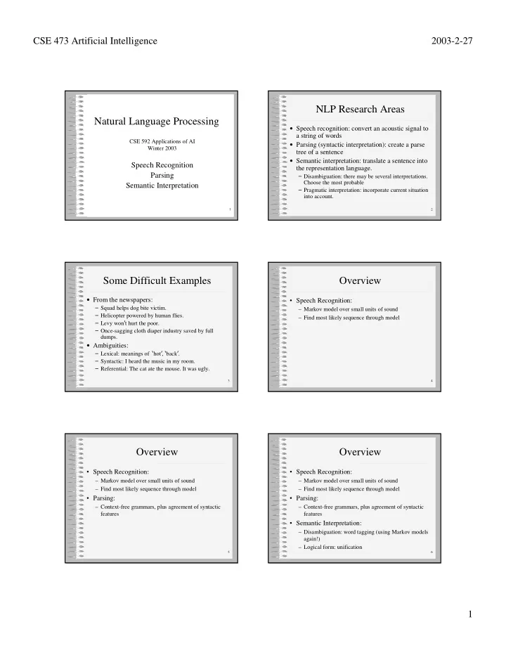
NLP Research Areas Natural Language Processing Speech recognition: - PDF document

CSE 473 Artificial Intelligence 2003-2-27 NLP Research Areas Natural Language Processing • Speech recognition: convert an acoustic signal to a string of words CSE 592 Applications of AI • Parsing (syntactic interpretation): create a parse Winter 2003 tree of a sentence • Semantic interpretation: translate a sentence into Speech Recognition the representation language. Parsing – Disambiguation: there may be several interpretations. Choose the most probable Semantic Interpretation – Pragmatic interpretation: incorporate current situation into account. 1 2 Some Difficult Examples Overview • From the newspapers: • Speech Recognition: – Squad helps dog bite victim. – Markov model over small units of sound – Helicopter powered by human flies. – Find most likely sequence through model – Levy won ’ t hurt the poor. – Once-sagging cloth diaper industry saved by full dumps. • Ambiguities: – Lexical: meanings of ‘ hot ’ , ‘ back ’ . – Syntactic: I heard the music in my room. – Referential: The cat ate the mouse. It was ugly. 3 4 Overview Overview • Speech Recognition: • Speech Recognition: – Markov model over small units of sound – Markov model over small units of sound – Find most likely sequence through model – Find most likely sequence through model • Parsing: • Parsing: – Context-free grammars, plus agreement of syntactic – Context-free grammars, plus agreement of syntactic features features • Semantic Interpretation: – Disambiguation: word tagging (using Markov models again!) – Logical form: unification 5 6 1

CSE 473 Artificial Intelligence 2003-2-27 Speech Recognition Difficulties ! Human languages are limited to a set of about ! Why isn't this easy? 40 to 50 distinct sounds called phones: e.g., – just develop a dictionary of pronunciation – [ey] bet e.g., coat = [k] + [ow] + [t] = [kowt] – [ah] but – but: recognize speech ≈ wreck a nice beach – [oy] boy ! Problems: – [em] bottom – homophones: different fragments sound the same – [en] button ! e.g., rec and wreck – segmentation: determining breaks between words ! These phones are characterized in terms of ! e.g., nize speech and nice beach acoustic features, e.g., frequency and amplitude, – signal processing problems that can be extracted from the sound waves 7 8 Speech Recognition Architecture Signal Processing ! Sound is an analog energy source resulting from � ����������������������������������������������� pressure waves striking an eardrum or microphone ������������������������������� ! A device called an analog-to-digital converter can Speech be used to record the speech sounds Waveform ������������������ – sampling rate: the number of times per second that ������������������� Spectral the sound level is measured Neural Net Feature Vectors – quantization factor: the maximum number of bits of ���������������� ��������������������� precision for the sound level measurements ������������������� Phone – e.g., telephone: 3 KHz (3000 times per second) N-gram Grammar Likelihoods P(o|q) – e.g., speech recognizer: 8 KHz with 8 bit samples ����������������� HMM Lexicon ����������������� so that 1 minute takes about 500K bytes 9 10 Words Signal Processing Signal Processing • Goal is speaker independence so that ! Wave encoding: – group into ~10 msec frames (larger blocks) that representation of sound is independent of a are analyzed individually speaker's specific pitch, volume, speed, etc. – frames overlap to ensure important acoustical and other aspects such as dialect events at frame boundaries aren't lost ! Speaker identification does the opposite, – frames are analyzed in terms of features, e.g., i.e. the specific details are needed to decide ! amount of energy at various frequencies who is speaking ! total energy in a frame ! A significant problem is dealing with background ! differences from prior frame noises that are often other speakers – vector quantization further encodes by mapping frame into regions in n-dimensional feature space 11 12 2

CSE 473 Artificial Intelligence 2003-2-27 Speech Recognition Model Language Model (LM) ! Bayes‘s Rule is used break up the problem into " P(words) is the joint probability that a sequence manageable parts: of words = w 1 w 2 ... w n is likely for a specified natural language P(words |signal) = P(words)P(signal| words) P(signal) ! This joint probability can be expressed using the chain rule (order reversed): – P(signal) : is ignored (normalizing constant ) P(w 1 w 2 … w n ) = P(w 1 ) P(w 2 | w 1 ) P(w 3 | w 1 w 2 ) ... P(w n | w 1 ... w n-1 ) – P(words) : Language model ! likelihood of words being heard ! Collecting the probabilities is too complex; it requires ! e.g. "recognize speech" more likely than "wreck a nice beach" statistics for m n-1 starting sequences for – P(signal | words) : Acoustic model a sequence of n words in a language of m words ! likelihood of a signal given words ! Simplification is necessary ! accounts for differences in pronunciation of words ! e.g . given "nice", likelihood that it is pronounced [nuys] etc. 13 14 Language Model (LM) Language Model (LM) ! First-order Markov Assumption says the probability ! More context could be used, such as the two words of a word depends only on the previous word: before, called the trigram model, but it's difficult to collect sufficient data to get accurate probabilities w 1 ... w i-1 ) ≈ ≈ P(w i | w P(w i | ≈ ≈ i-1 ) ! A weighted sum of unigram, bigram, trigram models could be used as a good combination: ! The LM simplifies to P(w 1 w 2 … w n ) = c 1 P(w i ) + c 2 P(w i | w i-1 ) + c 3 P(w i | w i-1 w i-2 ) P(w 1 w 2 … w n ) = P(w 1 ) P(w 2 | w 1 ) P(w 3 | w 2 ) ... P(w n | w n-1 ) ! Bigram and trigram models account for: – local context-sensitive effects – called the bigram model ! e.g. "bag of tricks" vs. "bottle of tricks" – it relates consecutive pairs of words – some local grammar ! e.g. "we was" vs. "we were" 15 16 Language Model (LM) Language Model (LM) ! Probabilities are obtained by computing statistics ! Probabilistic finite state of the frequency of all possible pairs of words in a machine: a (almost) fully attack large training set of word strings : connected directed graph: – if "the" appears in training data 10,000 times tomato the and it's followed by "clock" 11 times then ! nodes (states): all possible words P(clock| the) = 11/10000 = .0011 and a START state START of ! These probabilities are stored in: ! arcs: labeled with a probability – a probability table killer – from START to a word is the – a probabilistic finite state machine prior probability of the destination word – from one word to another is the probability ! Good-Turing estimator: of the destination word given the source word – total mass of unseen events ≈ total mass of events seen a single time 17 18 3