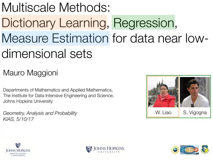
Multiscale Methods: Dictionary Learning, Regression, Measure - PowerPoint PPT Presentation

Multiscale Methods: Dictionary Learning, Regression, Measure Estimation for data near low ‐ dimensional sets Mauro Maggioni Departments of Mathematics and Applied Mathematics, The Institute for Data Intensive Engineering and Science, Johns Hopkins University W. Liao S. Vigogna Geometry, Analysis and Probability KIAS, 5/10/17

Curse of dimensionality Data as samples { x i } n i =1 from a probability distribution µ in R D In 1 dimension estimating µ could correspond to having a histogram where the height of a column in a bin is the probability of seeing a point in that bin. To estimate this histogram with accuracy ✏ , under reasonable conditions we need bins of width ✏ and at least constant number of points in each bin, for a total of O ( ✏ − 1 ) points. Unfortunately in D dimensions, there are O ( ✏ − D ) boxes of size ✏ . So we need O ( ✏ − D ) points. This is way too many: for ✏ = 10 − 1 and D = 100, we would need 10 100 points. ⊗ ⊗ ⊗ ⊗ ⊗ · · · Can we reduce the dimensionality?

“ In high dimensions ti ere are no fv nc tj ons, only measures ” P.W. Jones

Learning Geometry, Measure & Functions µ a probability measure in R D , D large. Assume that µ is (nearly) low- dimensional, e.g. concentrates around a manifold M of dimension d ⌧ D . Given n samples x 1 , . . . , x n i.i.d. from µ : · construct an e ffi cient encoding for samples from µ , i.e. a map D : R D → c i r R m , an inverse map D − 1 : R m → R D , such that: t e m m e o l e b G o r P x ∼ µ || x − D − 1 D ( x ) || 2 < ✏ . m = m ( ✏ ) is small x ∼ µ ||D ( x ) || 0 ≤ k , sup sup e 
 r u n s o · given just the x i ’s, construct ˆ µ close to µ . a i t e a M m i t s E · in addition given y i = f ( x i ) + η i , with η i independent of each other and n o i s of x i , construct ˆ f : R D → R such that P x ∼ µ ( || f ( x ) − ˆ s f ( x ) || L 2 ( µ ) > t ) is e r g e R small. \noindent $\mu$ a probability measure Objective: in $\mathbb{R}^D$, $D$ large. \noindent Objective: Assume that $\mu$ is (nearly) low- · Adaptive: no need to know regularity & fast algorithms: ˜ dimensional, e.g. concentrates around a O ( n ) or better. \noindent$\cdot$ Adaptive: no need to manifold $\mathcal{M}$ of dimension know regularity \& fast algorithms: $ · performance guarantees that depend on n (or ✏ ) and d , but no curse of ambient \tilde O(n)$ or better. dimensionality ( D ).

Principal Component Analysis 15 system of 10 coordinates U : orthogonal D × D 5 for points 0 Σ : diagonal D × n − 5 Diagonal entries σ 1 ≥ σ 2 ≥ · · · ≥ 0 − 10 are called singular values. − 15 − 10 − 5 0 5 10 15 20 V : orthogonal n × n system of coordinates for features 1901, K. Pearson

Intrinsic Dimension of Data

A. Little, MM, L. Rosasco, A.C.H.A. Model: data { x i } n i =1 is sampled from a manifold M of dimension k , embed- ded in R D , with k ⌧ D . We receive ˜ X n := { x i + η i } n i =1 , where η i ⇠ i . i . d N is D -dimensional noise (e.g. Gaussian). Objective: estimate k . ⇣ ( β 2 2 ,i � β 2 2 ,i +1 ) r 2 √ || η || ∼ σ D M z B r ( z ) M + η Green: where data is Red: where noisy data is Blue: volume in ball

Model: data { x i } n i =1 is sampled from a manifold M of dimension k , embed- ded in R D , with k ⌧ D . We receive ˜ X n := { x i + η i } n i =1 , where η i ⇠ i . i . d N is D -dimensional noise (e.g. Gaussian). Objective: estimate k . √ √ √ || η || ∼ σ || η || ∼ σ || η || ∼ σ D D D Green: where data is Red: where noisy data is M M M Blue: volume in ball z z z B r ( z ) M + η M + η M + η B r ( z ) B r ( z )

Multiscale SVD: sphere+noise Example: consider S 9 (100 , 1000 , 0 . 1): 1000 points uniformly samples on a 9- dimensional unit sphere, embedded in 100 dimensions, with Gaussian noise N (0 , 0 . 1 I 100 ). Observe that E [ || η || 2 ] ∼ 0 . 1 2 · 100 = 1. Small scales Large scales

Example: Molecular Dynamics Data Joint with C. Clementi, M. Rohrdanz, W. Zheng The dynamics of a small peptide (12 atoms with H -atoms removed) in a bath of water molecules, is approximated by a Langevin system of stochastic equations x = �r U ( x ) + ˙ ˙ w The set of configurations is a point cloud in R 12 × 3 . ψ φ

Example: Alanine dipeptide M. Rohrdanz, W. Zheng, MM, C. Clementi, J. Chem. Phys. 2011 ψ 0.4 Singular values 0.3 φ 0.2 Free energy in terms of MSVD near 0.1 empirical coordinates transition state 0 0.2 0.3 0.4 0.5 0.6 0.08 Singular values 0.06 MSVD near free 0.04 energy minimum 0.02 0 0.1 0.13 0.16 0.19 0.22 ε (˚ A )

Geometric MultiResolution Analysis W.K. Allard, G. Chen, MM, A.C.H.A. We are developing a multiscale geometric approximation for a point clouds M . We proceed in 3 stages: (i) Construct multiscale partitions {{ C j,k } k ∈ Γ j } J j =0 of the data: for each j , M = [ k ∈ Γ j C j,k , and C j,k is a nice “cube” at scale 2 − j . We obtain C j,k using cover trees. (ii) Compute low-rank SVD of the local covariance: cov j,k = Φ j,k Σ j,k Φ T j,k . Let P j,k be the a ffi ne projection R D ! V j,k := h Φ j,k i (local approxi- mate tangent space): P j,k ( x ) = Φ j,k Φ ∗ j,k ( x � c j,k ) + c j,k . These pieces of planes P j,k ( C j,k ) form an approximation M j to the original data M ; let P M j ( x ) := P j,k ( x ) for x 2 C j,k . (iii) We e ffi ciently encode the di ff erence Q M j +1 between P M j +1 ( x ) and P M j ( x ), by constructing a ffi ne “detail” operators analogous to the wavelet projections in wavelet theory. We obtain a multiscale nonlinear transform mapping data to a multiscale family of pieces of planes. Fast algorithms and multiscale organization allow for fast pruning and optimization algorithms to be run on this multiscale structure.

Geometric MultiResolution Analysis Scale from coarse to fine Subset of data j C j,k k Clusters at each scale

Geometric MultiResolution Analysis W.K. Allard, G. Chen, MM, A.C.H.A. We are developing a multiscale geometric approximation for a point clouds M . We proceed in 3 stages: (i) Construct multiscale partitions {{ C j,k } k ∈ Γ j } J j =0 of the data: for each j , M = [ k ∈ Γ j C j,k , and C j,k is a nice “cube” at scale 2 − j . We obtain C j,k using cover trees. (ii) Compute low-rank SVD of the local covariance: cov j,k = Φ j,k Σ j,k Φ T j,k . Let P j,k be the a ffi ne projection R D ! V j,k := h Φ j,k i (local approxi- mate tangent space): P j,k ( x ) = Φ j,k Φ ∗ j,k ( x � c j,k ) + c j,k . These pieces of planes P j,k ( C j,k ) form an approximation M j to the original data M ; let P M j ( x ) := P j,k ( x ) for x 2 C j,k . (iii) We e ffi ciently encode the di ff erence Q M j +1 between P M j +1 ( x ) and P M j ( x ), by constructing a ffi ne “detail” operators analogous to the wavelet projections in wavelet theory. We obtain a multiscale nonlinear transform mapping data to a multiscale family of pieces of planes. Fast algorithms and multiscale organization allow for fast pruning and optimization algorithms to be run on this multiscale structure.

Geometric MultiResolution Analysis M = ∪ k ∈ Γ j C j,k Local linear low-d approximation on piece of data Scale from coarse to fine h Φ j − 1 ,x i Subset of data j C j,k h Φ j,x i M j = ∪ k ∈ Γ j P j,k ( C j,k ) | {z } ⊆ V j,k x ∈ V J,x k Clusters at each scale

Geometric MultiResolution Analysis W.K. Allard, G. Chen, MM, A.C.H.A. We are developing a multiscale geometric approximation for a point clouds M . We proceed in 3 stages: (i) Construct multiscale partitions {{ C j,k } k ∈ Γ j } J j =0 of the data: for each j , M = [ k ∈ Γ j C j,k , and C j,k is a nice “cube” at scale 2 − j . We obtain C j,k using cover trees. (ii) Compute low-rank SVD of the local covariance: cov j,k = Φ j,k Σ j,k Φ T j,k . Let P j,k be the a ffi ne projection R D ! V j,k := h Φ j,k i (local approxi- mate tangent space): P j,k ( x ) = Φ j,k Φ ∗ j,k ( x � c j,k ) + c j,k . These pieces of planes P j,k ( C j,k ) form an approximation M j to the original data M ; let P M j ( x ) := P j,k ( x ) for x 2 C j,k . (iii) We e ffi ciently encode the di ff erence Q M j +1 between P M j +1 ( x ) and P M j ( x ), by constructing a ffi ne “detail” operators analogous to the wavelet projections in wavelet theory. We obtain a multiscale nonlinear transform mapping data to a multiscale family of pieces of planes. Fast algorithms and multiscale organization allow for fast pruning and optimization algorithms to be run on this multiscale structure.

Geometric MultiResolution Analysis M = ∪ k ∈ Γ j C j,k Local linear low-d approximation on piece of data Scale from coarse to fine h Φ j − 1 ,x i Subset of data h Ψ j,x i j C j,k h Φ j,x i M j = ∪ k ∈ Γ j P j,k ( C j,k ) | {z } ⊆ V j,k x ∈ V J,x k Clusters at each scale