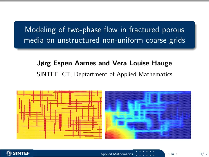
Modeling of two-phase flow in fractured porous media on unstructured - - PowerPoint PPT Presentation

Modeling of two-phase flow in fractured porous media on unstructured non-uniform coarse grids

Jørg Espen Aarnes and Vera Louise Hauge

SINTEF ICT, Deptartment of Applied Mathematics

Applied Mathematics 1/17

Objective and model assumptions

Objective: Develop an algorithm for constructing coarse grids capable of resolving two-phase flow in fractured porous media accurately. Model assumptions: Statistically generated horizontal and vertical fractures with length between 20–40% of length of shortest side of reservoir. Velocity computed on a fine grid that resolves fractures. Saturation computed on an unstructured coarse grid.

Homogeneous model with 100 fractures Heterogeneous model with 100 fractures

Applied Mathematics 2/17

Non-uniform coarsening algorithm

1 Compute the initial velocity field v on the fine grid and define

g(E) = 1 |E|

• E

log |v(x)| dx − min(log |v|) + 1, E ⊂ Ω.

2 Assign an integer from 1 to 10 to each cell c in the fine grid by

n(c) = ceil

• 10(g(c) − min

c g)/(max c

g − min

c g)

• .

3 Initial blocks = connected groups of cells with the same n(c). 4 Merge each block B with less volume than Vmin with

B′ = arg min

B′′∈neighbors |g(B) − g(B′′)|.

5 Refine each block B with |B|g(B) > Gmax as follows 1

Pick an arbitrary cell c0 ⊂ B and locate the cell ci ⊂ B with center furthest away from the center of c0.

2

Define B′ = ci and progressively enlarge B′ by adding cells from B adjacent to cells in B′ until |B′|g(B′) > Gmax.

3

Define B = B\B′ and refine B further if |B|g(B) > Gmax.

6 Repeat step 2 and terminate. Applied Mathematics 3/17

Non-uniform coarsening algorithm

Coarse grid: Initial step, 152 cells Coarse grid: Step 2, 47 cells Coarse grid: Step 3, 95 cells Coarse grid: Step 4, 69 cells

log |v| on fine grid (2500 cells) log |v| on coarse grid (69 cells)

Applied Mathematics 4/17

Explicit Fracture-Matrix Separation (EFMS)

1 2 2 1 3 4 2 1

Initial model: 100 x 100 grid with 50 fractures. Step 1: Introduce an initial coarse grid. Step 2: Separate fractures and matrix. Step 3: Split non-connected blocks.

Applied Mathematics 5/17

Operator splitting of saturation equation

Water saturation equation for a water-oil system: φ∂S ∂t + ∇ · [fw (v + λo∇pcow + λog(ρo − ρw)∇z)] = qw, Operator splitting of the water saturation equation φ∂S ∂t + ∇ · (fwv + fwλog(ρo − ρw)∇z) = qw, φ∂S ∂t + ∇ ·

• fwλo

∂pcow dS ∇S

• =

0.

Applied Mathematics 6/17

Numerical discretization of advection equation

Denote the non-degenerate fine grid interfaces by γij = ∂Ti ∩ ∂Tj. S

n+ 1

2

m

= Sn

m +

∆t

• Bmφ dx

 

• Bm

qw dx −

• γij⊂∂Bm

Vij(Sn+ 1

2 ) − Gij(Sn+ 1 2 )

  . Here Vij(S) = max{vijfw(S|Ti), − vijfw(S|Tj)}, Gij(S) = g(ρo − ρw)|γij| λw(S+)λo(S−) λw(S+) + λo(S−)∇z · nij, where vij = flux from Ti to Tj, nij = unit normal on γij from Ti to Tj, and S+ and S− is the upstream saturation with respect to the gravity driven flow of oil and water, respectively.

Applied Mathematics 7/17

Numerical example: Pure advective flow

Coarsening algorithm # blocks L2 water-cut error Non-uniform coarsening 255 0.0240 EFMS 315 0.1428 Cartesian coarse grid 330 0.1838 Saturation profiles at 0.48 PVI Reference solution NUC solution EFMS solution Cartesian solution Water-cut curves

0.2 0.4 0.6 0.8 1 0.2 0.4 0.6 0.8 1 PVI

Reference NUC EFMS Cartesian

Applied Mathematics 8/17

Test-case I: No capillary diffusion

100 high permeable fractures and 20 low permeable fractures. Permeability of high permeable fractures: > matrix permeability. Permeability of low permeable fractures: ≪ matrix permeability. 25 simulations with different fracture distributions. Homogeneous model Heterogeneous model

36 : 38 20 : 24 9 : 11 0.05 0.1 0.15 0.2 Upscaling factors Mean error Mean water−cut errors for homogeneous model EFMS NUC 40 : 47 19 : 21 6 : 9 0.05 0.1 0.15 0.2 0.25 Upscaling factors Mean error Mean water−cut errors for heterogeneous model EFMS NUC

Applied Mathematics 9/17

Numerical discretization of diffusion equation

Diffusion equation: φ∂S ∂t = ∇ · d(S)∇S, where d(S) = −fwλo

∂pcow dS

is a non-negative function. Time discretization: Semi-implicit backward Euler φSn+1 = φSn+1/2 + △t∇ · d(Sn+1/2)∇Sn+1. Spatial discretization: ??? How should △t∇ · d(Sn+1/2)∇Sn+1 be discretized on coarse grids with complex block geometries and strong subgrid heterogeneity?

Applied Mathematics 10/17

Spatial discretization of diffusion equation

Option 1: Fine grid discretization (Φ + △tD) Sn+1 = ΦSn+1/2, where Φ = diag(φ) and D = [dij(S)] stems from a fine grid discretization of the semi-elliptic operator L = ∇ · d∇.

Applied Mathematics 11/17

Spatial discretization of diffusion equation

Option 1: Fine grid discretization (Φ + △tD) Sn+1 = ΦSn+1/2, where Φ = diag(φ) and D = [dij(S)] stems from a fine grid discretization of the semi-elliptic operator L = ∇ · d∇. Option 2: Coarse grid discretization by Galerkin projection (Φc + △tDc) Sn+1

c

= ΦcSn+1/2

c

, where Φc = RtΦR and Dc = RtDR. Here R = [rij] where rij = 1 if cell i is contained in block j,

• therwise.

Hence, R maps coarse grid saturations onto the fine grid.

Applied Mathematics 11/17

Spatial discretization of diffusion equation

Orthogonal projection property If Sn+1 solves the fine grid system with Sn+1/2 = RSn+1/2

c

, then R(Sn+1

c

− Sn+1/2

c

) = arg min

Sc RSc − Sn+1,

where S = (S, (Φ + △tD)S)1/2, i.e., Sn+1

c

is the optimal coarse grid approximation to Sn+1 in the norm · .

Applied Mathematics 12/17

Spatial discretization of diffusion equation

Orthogonal projection property If Sn+1 solves the fine grid system with Sn+1/2 = RSn+1/2

c

, then R(Sn+1

c

− Sn+1/2

c

) = arg min

Sc RSc − Sn+1,

where S = (S, (Φ + △tD)S)1/2, i.e., Sn+1

c

is the optimal coarse grid approximation to Sn+1 in the norm · . The fine grid discretization gives too much diffusion! Gradients of the blockwise constant saturation is computed at the fine grid level: Options 1 and 2 overestimate diffusion.

Applied Mathematics 12/17

Spatial discretization of diffusion equation

The overestimation factor scales with the ratio of the size of the coarse grid blocks relative to the size of the fine grid cells. On average the diffusion should be damped by a factor (Nb/Nc)1/d, where Nb = number of blocks and Nc = number of cells.

Applied Mathematics 13/17

Spatial discretization of diffusion equation

The overestimation factor scales with the ratio of the size of the coarse grid blocks relative to the size of the fine grid cells. On average the diffusion should be damped by a factor (Nb/Nc)1/d, where Nb = number of blocks and Nc = number of cells. Scaled Galerkin projection

• Φc + △t

Nb Nc 1/d Dc

• Sn+1

c

= ΦcSn+1/2

c

.

Applied Mathematics 13/17

Test-case II: With capillary diffusion

Homogeneous model Heterogeneous model fine grid G. proj. scl. proj. fine grid G. proj. scl. proj. EFMS 0.071 0.077 0.028 0.091 0.107 0.051 NUC 0.047 0.055 0.079 0.063 0.109 0.033

0.2 0.4 0.6 0.8 1 0.2 0.4 0.6 0.8 1 Water−cut curves for homogeneous model Reference NUC (fine) NUC (coarse+scaling) NUC (coarse) 0.2 0.4 0.6 0.8 1 0.2 0.4 0.6 0.8 1 Water−cut curves for homogeneous model Reference EFMS (fine) EFMS (coarse+scaling) EFMS (coarse) 0.2 0.4 0.6 0.8 1 0.2 0.4 0.6 0.8 1 Water−cut curves for heterogeneous model Reference NUC (fine) NUC (coarse+scaling) NUC (coarse) 0.2 0.4 0.6 0.8 1 0.2 0.4 0.6 0.8 1 Water−cut curves for heterogeneous model Reference EFMS (fine) EFMS (coarse+scaling) EFMS (coarse)

Applied Mathematics 14/17

Test-case II: With capillary diffusion

Homogeneous model with 100 high permeable fractures: Saturation profiles at 0.2 PVI

Fracture model Reference solution NUC: fine grid diffusion EFMS: fine grid diffusion NUC: scaled G. projection EFMS: scaled G. projection

Applied Mathematics 15/17

Test-case II: With capillary diffusion

Heterogeneous model with 100 high permeable fractures: Saturation profiles at 0.2 PVI

Fracture model Reference solution NUC: fine grid diffusion EFMS: fine grid diffusion NUC: scaled G. projection EFMS: scaled G. projection

Applied Mathematics 16/17

Summary

For flows without capillary diffusion we consistently obtain significantly more accurate solutions on non-uniform coarse grids than on grids with explicit fracture-matrix separation. For flows with relatively strong capillary diffusion, the coarsening algorithms give comparable results for homogeneous fracture models, but non-uniform coarsening gives best results for heterogeneous fracture models. The scaled Galerkin projection generally models diffusion well

• n complex coarse grids, but more rigorous ways of damping

the fine scale diffusion will be studied in further research.

Applied Mathematics 17/17