[PDF] - MODEL BASED GEOSTATISTICS (Course Slides) Presented by: Paulo PDF Document

SLIDE 1

MODEL BASED GEOSTATISTICS

(Course Slides) Presented by: Paulo Justiniano Ribeiro Jr 1 Departamento de Estat´ ıstica Universidade Federal do Paran´ a, Brasil

1Correspondence Addrees: Departamento de Estat´

ıstica, Universidade Federal do Paran´ a, Cx. Pos- tal 19.081, 81.531-990, Curitiba, PR, Brasil. E-mail: pj@est.ufpr.br

SLIDE 2

Acknowledgements

The course notes and slides are result of joint work with:

Professor Peter J. Diggle

Department of Mathematics and Statistics Lancaster University, UK

Ole Christensen

Center for Bioinformatik, Datalogisk Institut, Aarhus Universitet, Denmark formlely at: Department of Mathematics and Statistics, Lancaster University, UK and Department of Mathematical Sciences, Aalborg University, Den- mark

SLIDE 3

PART I: INTRODUCTION

1. Basic Examples of Spatial Data
2. A Taxonomy for Spatial Statistics
3. Further Examples of Geostatistical Problems
4. Characteristic Features of Geostatistical Problems
5. Some History
6. Core Geostatistical Problems
7. Model Based Geostatistics

SLIDE 4

1. Basic Examples of Spatial Data

(a) Cancer rates in administrative regions Grey-scale corresponds to estimated varia- tion in relative risk of colorectal cancer in the 36 electoral wards of the city of Birmingham, UK.

395000 400000 405000 410000 415000 420000 275000 280000 285000 290000 295000 300000

Eastings (meters) Northings (meters)

0.9 1.0 1.1 1.2 1.3

2

SLIDE 5

(b) Rainfall in Paran´ a State, Brasil Rainfall measurements at 143 recording sta- tions. Average for the May-June period (dry sea- son).

200 300 400 500 600 700 800 100 200 300 400 500 600 E−W (km) N−S (km) 3

SLIDE 6

(c) Campylobacter cases in southern En- gland Residential locations of 651 cases of campylo- bacter reported over a one-year period in cen- tral southern England.

•
•
•
• •
•
•
••
•
••
•
•
•
•
•
•
•
•
•
•
• •
•
•
•
•
•
E-W (km)

N-S (km) 380 400 420 440 460 80 100 120 140

4

SLIDE 7

2. A Taxonomy of Spatial Statistics

(a) Discrete spatial variation Basic structure. Yi : i = 1, ..., n

rarely arises naturally
but often useful as a pragmatic strategy
models typically defined indirectly from

full conditionals, [Yi|Yj, ∀j = i] (b) Continuous spatial variation Basic structure. Y (x) : x ∈ I R2

data (yi, xi) : i = 1, ..., n, locations xi may be:

– non-stochastic (eg lattice to cover obser- vation region A) – or stochastic, but independent of the process Y (x) (c) Spatial point processes Basic structure. Countable set of points xi ∈ I R2, generated stochastically.

data sometimes converted to apparently

discrete spatial variation by aggregation

ver sub-regions

5

SLIDE 8

Spatial statistics is the collection of statisti- cal methods in which spatial locations play an explicit role in the analysis of data. Two strategic issues:

don’t confuse the data-format with the un-

derlying process

the choice of model may be influenced by the

scientific objectives of the study – analyse problems, not data

6

SLIDE 9

3. Further Examples of Geostatistical

Problems

(a) Swiss rainfall data

E-W (km) N-S (km) 100 200 300 50 100 150 200

Locations shown as points with size proportional to the value of the observed rainfall.

467 locations in Switzerland
daily rainfall measurements on 8th of May

1986

data from:

Spatial Interpolation Comparison 97 (ftp://ftp.geog.uwo.ca/SIC97/).

7

SLIDE 10

(b) Rongelap Island

study of residual contamination, following

nuclear weapons testing programme du- ring 1950’s

island evacuated in 1985, is it now safe for

re-settlement?

survey yields noisy measurements Yi of ra-

dioactive caesium concentrations

initial grid of locations xi at 200m spacing

later supplemented by in-fill squares at 40m spacing.

particular interest in maximum caesium

concentration

E-W N-S

6000
5000
4000
3000
2000
1000
5000
4000
3000
2000
1000

1000

•
•
• • •
• • • • • • • • • • • • • • • •• •
•
•
8

SLIDE 11

(c) Gambia malaria

survey of villages in Gambia
in village i, data Yij = 0/1 denotes ab-

sence/presence of malarial parasites in blood sample from child j

village-level covariates:

– village locations – public health centre in village? – satellite-derived vegetation green-ness index

child-level covariates:

– age, sex, bed-net use

interest in effects of covariates, and pat-

tern of residual spatial variation

E-W (km) N-S (km) 300 400 500 600 1400 1500 1600

o
Western

Eastern 300 400 500 600 1400 1500 1600

300

400 500 600 1400 1500 1600 Central

300

400 500 600 1400 1500 1600

o
9

SLIDE 12

4. Characteristic Features of Geosta-

tistical Problems

data consist of responses Yi associated with

locations xi

in principle, Y could be determined from any

location x within a continuous spatial region A

it is reasonable to behave as if {Y (x) : x ∈ A}

is a stochastic process

xi is typically fixed. If the locations xi are ge-

nerated by a stochastic point process, it is re- asonable to behave as if this point process is independent of the Y (x) process

scientific objectives include prediction of one
r more functionals of a stochastic process

{S(x) : x ∈ A} which is dependent on the Y (x) process.

10

SLIDE 13

5. Some History
Origins in problems connected with esti-

mation of ore reserves in mineral explora- tion/mining (Krige, 1951).

Subsequent development largely indepen-

dent of “mainstream” spatial statistics, initi- ally by Matheron and colleagues at ´ Ecole des Mines, Fontainebleau.

Parallel

developments by Mat´ ern (1946, 1960), Whittle (1954, 1962, 1963)

Ripley (1981) re-casts kriging in terminology
f stochastic process prediction
Significant cross-fertilization during 1980’s

and 1990’s (eg variogram is now a standard statistical tool for analysing correlated data in space and/or time).

But still vigorous debate on practical issues:

– prediction vs inference – role of explicit probability models

11

SLIDE 14

6. Core Geostatistical Problems
Design

– how many locations? – how many measurements? – spatial layout of the locations? – what to measure at each location?

Modelling

– probability model for the signal, [S] – conditional probability model for the mea- surements, [Y |S]

Estimation

– assign values to unknown model parame- ters – make inferences about (functions of) model parameters

Prediction

– evaluate [T|Y ], the conditional distribution

f the target given the data

12

SLIDE 15

7. Model-Based Geostatistics
declares explicit stochastic model
apply general statistical principles for infe-

rence Notation (Yi, xi) : i = 1, ..., n

{xi : i = 1, ..., n} is the sampling design
{Y (x) : x ∈ A} is the measurement process
{S(x) : x ∈ A} is the signal process
T = F(S) is the target for prediction
[S, Y ] = [S][Y |S] is the geostatistical model

13

SLIDE 16

Traditional geostatistics:

avoids explicit references to the parametric

specification of the model

inference via variograms

(Matheron’s “estimating and choosing”)

complex variogram structures are often used
concentrates on linear estimators
specific methods/paradigms for:

– point prediction (SK, OK, KTE, UK) – prediction of non-linear functionals (IK, DK) – predictive estimation (IK, DK) – simulations from the predictive distribu- tion (SGSIM, SISIM, ...)

the kriging menu

14

SLIDE 17

PART II: SPATIAL PREDICTION AND GAUSSIAN MODELS

1. The Gaussian Model
2. Specification of the Correlation Function
3. Stochastic Process Prediction
4. Linear Geostatistics
5. Prediction under the Gaussian Model
6. What does Kriging Actually do to the Data
7. Prediction of Functionals
8. Directional Effects
9. Non-stationary Gaussian Models

SLIDE 18

1. The Gaussian Spatial Model

(a) S(·) is a stationary Gaussian process with

i. E[S(x)] = µ,
ii. Var{S(x)} = σ2
iii. ρ(u) = Corr{S(x), S(x − u)};

(b) the conditional distribution of Yi given S(·) is Gaussian with mean S(xi) and variance τ 2; (c) Yi : i = 1, ..., n are mutually independent, con- ditional on S(·).

0.0 0.2 0.4 0.6 0.8 1.0 4.0 4.5 5.0 5.5 6.0 6.5 7.0 locations data

simulated data in 1-D illustrating the elements of the mo- del: data Y (xi) (dots), signal S(x) (curve line) and mean µ. (horizontal line).

16

SLIDE 19

An Equivalent Formulation: Yi = S(xi) + i : i = 1, ..., n. where i : i = 1, ..., n are mutually independent, identically distributed with i ∼ N(0, τ 2). Then, the joint distribution of Y is multivariate Normal, Y ∼ MVN(µ1, σ2R + τ 2I) where: 1 denotes an n-element vector of ones, I is the n × n identity matrix R is the n × n matrix with (i, j)th element ρ(uij) where uij = ||xi − xj||, the Euclidean distance between xi and xj.

17

SLIDE 20

2. Specification
f

the Correlation Function

Differentiability of Gaussian processes

A formal mathematical description of the

smoothness of a spatial surface S(x) is its de- gree of differentiability.

A process S(x) is mean-square continuous if,

for all x, E[{S(x + h) − S(x)}2] → 0 as h → 0.

S(x) is mean square differentiable if there

exists a process S′(x) such that, for all x, E S(x + h) − S(x) h − S′(x) 2 → 0 as h → 0

the mean-square differentiability of S(x) is

directly linked to the differentiability of its covariance function Theorem 3 Let S(x) be a stationary Gaussian process with correlation function ρ(u) : u ∈ I R. Then:

S(x) is mean-square continuous iff ρ(u) is con-

tinuous at u = 0;

S(x) is k times mean-square differentiable iff

ρ(u) is (at least) 2k times differentiable at u = 0.

18

SLIDE 21

(a) The Mat´ ern family The correlation function is given by: ρ(u) = {2κ−1Γ(κ)}−1(u/φ)κKκ(u/φ)

κ and φ are parameters
Kκ(·) denotes modified Bessel function of
rder κ
valid for φ > 0 and κ > 0.
κ = 0.5: exponential correlation function
κ → ∞: Gaussian correlation function
S(x) is mean-square ⌈κ − 1 times differen-

tiable

0.0 0.2 0.4 0.6 0.8 1.0 0.0 0.2 0.4 0.6 0.8 1.0 distance correlation

Three examples of the Mat´ ern correlation function with φ = 0.2 and κ = 1 (solid line), κ = 1.5 (dashed line) and κ = 2 (dotted line).

19

SLIDE 22

(b) The powered exponential family ρ(u) = exp{−(u/φ)κ}

defined for φ > 0 and 0 < κ ≤ 2
φ and κ are parameters
mean-square

continuous (but non- differentiable) if κ < 2

mean-square infinitely differentiable if κ =

2

ρ(u) very ill-conditioned when κ = 2
κ = 1: exponential correlation function
κ = 2: Gaussian correlation function

Conclusion: not as flexible as it looks

0.0 0.2 0.4 0.6 0.8 1.0 0.0 0.2 0.4 0.6 0.8 1.0 distance correlation

Three examples of the powered exponential correla- tion function with φ = 0.2 and κ = 1 (solid line), κ = 1.5 (dashed line) and κ = 2 (dotted line).

20

SLIDE 23

(c) The spherical family ρ(u; φ) = 1 − 3

2(u/φ) + 1 2(u/φ)3 : 0 ≤ u ≤ φ

: u > φ

φ > 0 is parameter
finite range
non-differentiable at the origin

0.0 0.2 0.4 0.6 0.8 1.0 0.0 0.2 0.4 0.6 0.8 1.0 distance correlation

The spherical correlation function with φ = 0.6.

21

SLIDE 24

Comparable Simulations (same seed)

0.0 0.2 0.4 0.6 0.8 1.0 −1.5 −1.0 −0.5 0.0 0.5 1.0 1.5 x y

simulations with Mat´ ern correlation functions with φ = 0.2 and κ = 0.5 (solid line), κ = 1 (dashed line) and κ = 2 (dotted line).

0.0 0.2 0.4 0.6 0.8 1.0 −1.5 −1.0 −0.5 0.0 0.5 1.0 1.5 x y

simulations with powered exponential correlation function with φ = 0.2 and κ = 1 (solid line), κ = 1.5 (dashed line) and κ = 2 (dotted line).

0.0 0.2 0.4 0.6 0.8 1.0 −1.5 −1.0 −0.5 0.0 0.5 1.0 1.5 x y

simulations with spherical correlation function (φ = 0.6).

22

SLIDE 25

3. Stochastic Process Prediction

General results for prediction goal: predict the realised value of a (scalar) r.v. T, using data y a realisation of a (vector) r.v. Y . predictor: of T is any function of Y , ˆ T = t(Y ) best choice: needs a criterion MMSPE: the best predictor minimises MSPE( ˆ T) = E[(T − ˆ T)2] Theorem 1. The minimum mean square error predictor of T is ˆ T = E(T|Y ). Theorem 2. (a) The prediction mean square error of ˆ T is E[(T − ˆ T)2] = EY [Var(T|Y )], (the prediction variance is an estimate of the MSPE). (b) E[(T − ˆ T)2] ≤ Var(T), with equality if T and Y are independent random variables.

23

SLIDE 26

Comments

We call ˆ

T the least squares predictor for T, and Var(T|Y ) its prediction variance

Var(T) − Var(T|Y ) measures the contribution
f the data (exploiting dependence between T

and Y )

point prediction,

prediction variance are summaries

complete answer is the distribution [T|Y ]
not transformation invariant:

ˆ T the best predictor for T does NOT necessa- rily imply that g( ˆ T) is the best predictor for g(T).

24

SLIDE 27

4. Linear Gaussian Geostatistics

Suppose the target for prediction is T = S(x) A predictor for T is a function ˆ T = ˆ T(Y ) The mean square prediction error (MSPE) is MSPE( ˆ T) = E[( ˆ T − T)2] The the predictor which minimises MSPE is ˆ T = E[S(x)|Y ] Two approaches:

Model-based geostatistics:

– specify a probability model for [Y, T] – choose ˆ T to minimise MSPE( ˆ T) amongst all functions ˆ T(Y )

Traditional (linear) geostatistics:

– Assume that ˆ T is linear in Y , so that ˆ T = b0(x) +

n

i=1

bi(x)Yi – Choose bi to minimise MSPE( ˆ T) within the class of linear predictors Coincident results under Gaussian assumpti-

ns

25

SLIDE 28

5. Prediction

Under The Gaussian Model

assume that the target for prediction is T =

S(x)

[T, Y ] are jointly multivariate Gaussian.
ˆ

T = E(T|Y ), Var(T|Y ) and [T|Y ] can be easily derived from a standard result: Theorem 4. Let X = (X1, X2) be jointly multi- variate Gaussian, with mean vector µ = (µ1, µ2) and covariance matrix Σ = Σ11 Σ12 Σ21 Σ22

,

ie X ∼ MVN(µ, Σ). Then, the conditional distri- bution of X1 given X2 is also multivariate Gaus- sian, X1|X2 ∼ MVN(µ1|2, Σ1|2), where µ1|2 = µ1 + Σ12Σ−1

22 (X2 − µ2)

and Σ1|2 = Σ11 − Σ12Σ−1

22 Σ21.

26

SLIDE 29

For the geostatistical model: [T, Y ] is multivariate Gaussian with mean vec- tor µ1 and variance matrix σ2 σ2r′ σ2r τ 2I + σ2R

where r is a vector with elements ri = ρ(||x −

xi||) : i = 1, ..., n. Hence, using Theorem 4 with X1 = T and X2 = Y , we find that the minimum mean square error predictor for T = S(x) is ˆ T = µ + σ2r′(τ 2I + σ2R)−1(Y − µ1) (1) with prediction variance Var(T|Y ) = σ2 − σ2r′(τ 2I + σ2R)−1σ2r. (2)

27

SLIDE 30

Notes

1. Because the conditional variance does not de-

pend on Y , the prediction mean square error is equal to the prediction variance.

2. Equality of prediction mean square error and

prediction variance is a special property of the multivariate Gaussian distribution, not a gene- ral result. 3. In conventional geostatistical terminology, construction of the surface ˆ S(x), where ˆ T = ˆ S(x) is given by (1), is called simple kriging. This name is a reference to D.G. Krige, who pionee- red the use of statistical methods in the South African mining industry (Krige, 1951).

28

SLIDE 31

6. What Does Kriging Actually Do to

the Data?

The minimum mean square error predictor for S(x) is given by ˆ T = ˆ S(x) = µ +

n

i=1

wi(x)(Yi − µ) = {1 −

n

i=1

wi(x)}µ +

n

i=1

wi(x)Yi

the predictor ˆ

S(x) compromises between its unconditional mean µ and the observed data Y

the nature of the compromise depends on the

target location x, the data-locations xi and the values of the model parameters.

call the wi(x) the prediction weights.

29

SLIDE 32

6.1 Effects on predictions

(a) Varying the correlation function

0.0 0.2 0.4 0.6 0.8 1.0 −2 −1 1 2 locations predicted signal

Predictions from 10 equally spaced data-points using expo- nential (solid line) or Mat´ ern of order 2 (dashed line) correla- tion functions.

0.0 0.2 0.4 0.6 0.8 1.0 −2.5 −2.0 −1.5 −1.0 −0.5 0.0 0.5 locations predicted signal

Predictions from 10 randomly spaced data-points using expo- nential (solid line) or Mat´ ern of order 2 (dashed line) correla- tion functions.

30

SLIDE 33

(b) Varying the correlation parameter

0.0 0.2 0.4 0.6 0.8 1.0 −0.5 0.0 0.5 1.0 1.5 2.0 locations predicted signal

Predictions from 10 randomly spaced data-points using the Mat´ ern (κ = 2) correlation function and different values of φ: 0.05 (solid line), 0.1 (dashed line) and 0.5 (thick dashed line).

31

SLIDE 34

(c) Varying the noise-to-signal ratio

0.0 0.2 0.4 0.6 0.8 1.0 −0.5 0.0 0.5 1.0 1.5 2.0 locations predicted signal

Predictions from 10 randomly spaced data-points using the Mat´ ern correlation function and different values of τ 2: 0 (solid line), 0.25 (dashed line) and 0.5 (thick dashed line).

0.0 0.2 0.4 0.6 0.8 1.0 0.0 0.1 0.2 0.3 0.4 locations prediction variance

Prediction variances from 10 randomly spaced data- points using the Mat´ ern correlation function and dif- ferent values of τ 2: 0 (solid line), 0.25 (dashed line) and 0.5 (thick dashed line).

32

SLIDE 35

6.2 Effects on kriging weights

(a) The prediction weights: varying φ

0.2 0.4 0.6 0.8 −0.2 0.0 0.2 0.4 0.6

φ = 0

data locations prediction weights 0.2 0.4 0.6 0.8 −0.2 0.0 0.2 0.4 0.6

φ = 0.05

data locations prediction weights 0.2 0.4 0.6 0.8 −0.2 0.0 0.2 0.4 0.6

φ = 0.15

data locations prediction weights 0.2 0.4 0.6 0.8 −0.2 0.0 0.2 0.4 0.6

φ = 0.3

data locations prediction weights

Prediction weights for 10 equally spaced data-points with tar- get location x = 0.50.

i. varying parameter φ = 0, 0.05, 0.15, 0.30
ii. locations: equally spaced xi = −0.05 + 0.1i :

i = 1, ..., 10

iii. prediction location: x = 0.50
iv. correlation function: Mat´

ern with κ = 2

v. nugget: τ 2 = 0

33

SLIDE 36

(b) The prediction weights: varying κ

0.2 0.4 0.6 0.8 −0.2 0.0 0.2 0.4 0.6

κ = 0.5

data locations prediction weights 0.2 0.4 0.6 0.8 −0.2 0.0 0.2 0.4 0.6

κ = 1

data locations prediction weights 0.2 0.4 0.6 0.8 −0.2 0.0 0.2 0.4 0.6

κ = 2

data locations prediction weights 0.2 0.4 0.6 0.8 −0.2 0.0 0.2 0.4 0.6

κ = 5

data locations prediction weights

Prediction weights for 10 equally spaced data-points with tar- get location x = 0.50.

i. varying parameter κ = 0.5, 1, 2, 5
ii. locations: equally spaced xi = −0.05 + 0.1i :

i = 1, ..., 10

iii. prediction location: x = 0.50
iv. correlation function: Mat´

ern with φ = 0.1

v. Nugget: τ 2 = 0

34

SLIDE 37

(c) The prediction weights: varying τ 2

0.2 0.4 0.6 0.8 0.0 0.4 0.8

τ2 = 0

data locations prediction weights 0.2 0.4 0.6 0.8 0.0 0.4 0.8

τ2 = 0.1

data locations prediction weights 0.2 0.4 0.6 0.8 0.0 0.4 0.8

τ2 = 0.25

data locations prediction weights 0.2 0.4 0.6 0.8 0.0 0.4 0.8

τ2 = 0.5

data locations prediction weights

Prediction weights for 10 equally spaced data-points with tar- get location x = 0.45.

i. varying parameter τ 2 = 0, 0.1, 0.25, 0.5
ii. locations: equally spaced xi = −0.05 + 0.1i :

i = 1, ..., 10

iii. prediction location: x = 0.45
iv. correlation function: Mat´

ern with κ = 2 and φ = 0.1

35

SLIDE 38

7. Prediction of Functionals

Let T be any linear functional of S, T =

A

w(x)S(x)dx for some prescribed weighting function w(x). Under the Gaussian model:

[T, Y ] is multivariate Gaussian;
[T|Y ] is univariate Gaussian;
the conditional mean and variance are:

E[T|Y ] =

A

w(x)E[S(x)|Y ]dx Var[T|Y ] =

A
A

w(x)w(x′)Cov{S(x), S(x′)}dxdx′ Note in particular that ˆ T =

A

w(x) ˆ S(x)dx

36

SLIDE 39

In words:

given a predicted surface ˆ

S(x), it is legitimate simply to calculate any linear property of this surface and to use the result as the predictor for the corresponding linear property of the true surface S(x)

it is NOT legitimate to do this for prediction
f non-linear properties
for example, the maximum of ˆ

S(x) is a very bad predictor for the maximum of S(x) (this problem will be addressed later)

37

SLIDE 40

8. Directional Effects
Environmental conditions can induce directi-
nal effects (wind, soil formation, etc).
As a consequence the spatial correlation may

vary with the direction.

0.1 0.2 0.3 0.4 0.5 0.6 0.7 0.8

−1.0 −0.5 0.0 0.5 1.0 −1.0 −0.5 0.0 0.5 1.0

. 1 0.2 . 3 0.4 0.5 0.6 0.7

−1.0 −0.5 0.0 0.5 1.0 −1.0 −0.5 0.0 0.5 1.0

. 1 0.2 0.3 . 4 0.5 0.6 . 7

−1.0 −0.5 0.0 0.5 1.0 −1.0 −0.5 0.0 0.5 1.0

correlation contours for a isotropic model (left) and two anisotropic models (center and right).

a possible approach: geometric anisotropy.
two more parameters: the anisotropy angle

ψA and the anisotropy ratio ψR.

rotation and stretching of the original coordi-

nates: (x1′, x2′) = (x1, x2) cos(ψA) − sin(ψA) sin(ψA) cos(ψA) 1

1 ψR

38

SLIDE 41

Geometric Anisotropy Correction

0.0 0.2 0.4 0.6 0.8 1.0 0.0 0.2 0.4 0.6 0.8 1.0

Original Space, ψ1 = 0°, ψ2 = 2

1 2 3 4 5 6 7 8 9 10 11 12 13 14 15 16 17 18 19 20 21 22 23 24 25 26 27 28 29 30 31 32 33 34 35 36 x 0.0 0.2 0.4 0.6 0.8 1.0 −0.2 0.0 0.2 0.4 0.6

Isotropic Space

1 2 3 4 5 6 7 8 9 10 11 12 13 14 15 16 17 18 19 20 21 22 23 24 25 26 27 28 29 30 31 32 33 34 35 36 x 0.0 0.2 0.4 0.6 0.8 1.0 0.0 0.2 0.4 0.6 0.8 1.0

Original Space, ψ1 = 120°, ψ2 = 2

1 2 3 4 5 6 7 8 9 10 11 12 13 14 15 16 17 18 19 20 21 22 23 24 25 26 27 28 29 30 31 32 33 34 35 36 x −1.4 −1.2 −1.0 −0.8 −0.6 −0.4 −0.2 0.0 −0.6 −0.4 −0.2 0.0 0.2 0.4 0.6 0.8

Isotropic Space

1 2 3 4 5 6 7 8 9 10 11 12 13 14 15 16 17 18 19 20 21 22 23 24 25 26 27 28 29 30 31 32 33 34 35 36 x 0.0 0.2 0.4 0.6 0.8 1.0 0.0 0.2 0.4 0.6 0.8 1.0

Original Space, ψ1 = 45°, ψ2 = 2

1 2 3 4 5 6 7 8 9 10 11 12 13 14 15 16 17 18 19 20 21 22 23 24 25 26 27 28 29 30 31 32 33 34 35 36 x −0.6 −0.4 −0.2 0.0 0.2 0.4 0.6 −0.4 −0.2 0.0 0.2 0.4 0.6 0.8 1.0

Isotropic Space

1 2 3 4 5 6 7 8 9 10 11 12 13 14 15 16 17 18 19 20 21 22 23 24 25 26 27 28 29 30 31 32 33 34 35 36 x

39

SLIDE 42

9. Non-Stationary Gaussian Models

Stationarity is a convenient working assump- tion, which can be relaxed in various ways.

Functional relationship between mean

and variance? Can sometimes be resolved by a transforma- tion of the data.

Non-constant mean?

Replace constant µ by µ(x) = Fβ =

k

j=1

βjfj(x) for measured covariates fj(x) (or non-linear versions). Note: sometimes called universal kriging

r kriging with external trend.

40

SLIDE 43

Non-stationary random variation?

Intrinsic variation a weaker hypothesis than stationarity (process has stationary in- crements, cf random walk model in time series), widely used as default model for discrete spatial variation (Besag, York and Moli´ e, 1991). Spatial deformation methods (Sampson and Guttorp, 1992) seek to achieve statio- narity by transformation of the geographical space, x.

as always, need to balance increased fle-

xibility of general modelling assumptions against over-modelling of sparse data, lea- ding to poor identifiability of model parame- ters.

41

SLIDE 44

PART III: PARAMETRIC ESTIMATION

1. Second-Moment Properties
2. Variogram Analysis
3. Likelihood Inference
4. Plug-in Prediction
5. Gaussian Transformed Models
6. A Case Study
7. Anisotropic Models
8. Model Validation

SLIDE 45

1. Second-Moment Properties
the variogram of a process Y (x) is the func-

tion V (x, x′) = 1 2Var{Y (x) − Y (x′)}

for the spatial Gaussian model, with u = ||x−

x′||, V (u) = τ 2 + σ2{1 − ρ0(u)}

basic structural parameters of the spatial

Gaussian model are: – the nugget variance: τ 2 – the sill: σ2 = Var{S(x)} – the total sill: τ 2 + σ2 = Var{Y (x)} – the range: φ, such ρ0(u) = ρ(u/φ)

practical implications:

– any reasonable version of the (linear) spa- tial Gaussian model has at least three pa- rameters – but you need a lot of data (or contextual knowledge) to justify estimating more than three parameters

the Mat´

ern family uses a fourth parameter to determine the differentiability of S(x)

43

SLIDE 46

Paradigmas for parameter estimation

Ad hoc (variogram based) methods

– compute the empirical variogram – fit a theoretical covariance model

Likelihood-based methods

– typically under Gaussian assumptions – Optimal under stated assumptions, but computationally expensive and may lack robustness?

Bayesian implementation,

combining estimation with prediction, beco- ming more widely accepted (amongst statis- ticians!)

44

SLIDE 47

2. Variogram Analysis
The variogram is defined by

V (x, x′) = 1 2Var{Y (x) − Y (x′)}

if Y (x) is stationary,

V (x, x′) = V (u) = 1 2E[{Y (x) − Y (x′)}2] where u = ||x − x′||

suggests an empirical estimate of V (u):

ˆ V (u) = average{[y(xi) − y(xj)]2} where each average is taken over all pairs [y(xi), y(xj)] such that ||xi − xj|| ≈ u

for a process with non-constant mean (cova-

riates), trend-removal can be used as follows: – define ri = Yi − ˆ µ(xi) – define ˆ V (u) = average{(ri − rj)2}, where each average is taken over all pairs (ri, rj)

45

SLIDE 48

(a) The variogram cloud

define the quantities

ri = Yi − ˆ µ(xi) uij = ||xi − xj|| vij = (ri − rj)2 2

the variogram cloud is a scatterplot of

the points (uij, vij) Example: Swiss rainfall data

50 100 150 200 50000 100000 150000 distance semivariance

under the spatial Gaussian model:

– vij ∼ V (uij)χ2

1

– the vij are correlated

the variogram cloud is therefore unstable,

both pointwise and in its overall shape

46

SLIDE 49

(b) The empirical variogram

derived from the variogram cloud by ave-

raging within bins: u−h/2 ≤ uij < u+h/2

forms k bins, each averaging over nk pairs
removes the first objection to the vario-

gram cloud, but not the second

is sensitive to mis-specification of µ(x)

Example: Swiss rainfall data.

50 100 150 200 5000 10000 15000 distance semivariance

Empirical binned variogram

47

SLIDE 50

(c) The fitted variogram Estimate ˜ θ to minimise a particular crite- rium eg, the weighted least squares (Cressie, 1993) S(θ) =

k

nk{[ ¯ Vk − V (uk; θ)]/V (uij; θ)}2 where ¯ Vk is average of nk variogram ordinates vij. Other criteria: OLS, WLS with weights given nk only, ...

Corresponds to biased estimating equation

for θ, although still widely used in practice.

Potentially misleading because of inherent

correlations amongst successive ¯ Vk Example: Swiss rainfall data

50 100 150 200 20 40 60 80 100 distance semivariance WLS 1 WLS 2 OLS

Empirical variogram with WLS with nk only (thick line), Cressie’s WLS (full line) and OLS (dashed line)

48

SLIDE 51

Further comments on empirical vario- grams

(a) Variograms of raw data and residuals can be very different Example: Paran´ a rainfall data.

• • •
• • •
•
•
100

200 300 400 1000 2000 3000 4000 5000 6000

• •
• •
• •
•
•
•

100 200 300 400 200 400 600 800 1000

empirical variograms of raw data (left-hand panel) and of residuals after linear regression on latitude, longitude and altitude (right-hand panel).

variogram of raw data includes variation

due to large-scale geographical trend

variogram of residuals eliminates this

source

f variation

49

SLIDE 52

(b) How unstable are empirical variograms?

Distance

Semi-variance 0.0 0.2 0.4 0.6 0.8 1.0 0.0 0.2 0.4 0.6 0.8 1.0

thick solid line shows true underlying va-

riogram

fine lines show empirical variograms from

three independent simulations of the same mo- del

high autocorrelations amongst

ˆ V (u) for successive values of u imparts misleading smoothness

50

SLIDE 53

3. Likelihood Inference

(a) Maximum likelihood estimation (ML) The Gaussian model is given by: Yi|S ∼ N(S(xi), τ 2)

S(xi) = µ(xi) + Sc(xi)
Sc(·) is a zero mean stationary Gaus-

sian process with covariance parameters (σ2, φ, κ),

µ(xi) = Fβ = k

j=1 fk(xi)βk, where fk(xi) is

a vector of covariates at location xi Which allows us to write: Yi = µ(xi) + Sc(xi) + i : i = 1, ..., n Then Y ∼ MVN(Fβ, σ2R + τ 2I) and the likelihood function is L(β, τ, σ, φ, κ) ∝ −0.5{log |(σ2R + τ 2I)| + (y − Fβ)′(σ2R + τ 2I)−1(y − Fβ)}. which maximisation yields the maximum li- kelihood estimates of the model parameters.

51

SLIDE 54

Maximum likelihood estimation (cont.) Computational details:

reparametrise ν2 = τ2

σ2 and denote:

σ2V = σ2(R + ν2I)

the log-likelihood function is maximised

for ˆ β(V ) = (F ′V −1F)−1F ′V −1y ˆ σ2 = n−1(y − F ˆ β)′V −1(y − F ˆ β)

then substituting (β, σ2) by ( ˆ

β, ˆ σ2) in 3 the maximisation reduces to L(τr, φ, κ) ∝ −0.5{n log | ˆ σ2| + log |(R + ν2I)|}

For the Mat´

ern correlation function we suggest to take κ in a discrete set {0.5, 1, 2, 3, ..., N}

52

SLIDE 55

(b) Restricted Maximum Likelihood Esti- mation (REML) The REML principle is as follows:

under the assumed model for E[Y ] = Fβ,

transform the data linearly to Y ∗ = AY such that the distribution of Y ∗ does not depend on β;

estimate θ = (ν2, σ2, φ, κ) by maximum like-

lihood applied to the transformed data Y ∗ We can always find a suitable matrix A without knowing the true values of β or θ, for example A = I − F(F ′F)−1F ′ The REML estimators for θ can be computed by maximising L∗(θ) ∝ −1 2

log |σ2V | + log |F ′{σ2V }−1F|

+(y − F ˜ β)′{σ2V }−1(y − F ˜ β))

,

where ˜ β = ˆ β(θ).

53

SLIDE 56

Comments on REML

introduced in the context of variance com-

ponents estimation in designed experi- ments (Patterson and Thompson, 1971)

leads to less biased estimators in small

samples

L∗(θ) depends on F, and therefore on a cor-

rect specification of the model for µ(x),

L∗(θ) does not depend on the choice of A.
Given the model for µ(·), the method enjoys

the same objectivity as does maximum li- kelihood estimation.

widely recommended for geostatistical mo-

dels.

REML is more sensitive than ML to mis-

specification of the model for µ(x).

for designed experiments the mean µ(x) is

usually well specified

however in the spatial setting there is no

sharp distinction between µ(x) and Sc(x).

54

SLIDE 57

Profile likelihood Variability of the parameter estimators can be inspected by looking at the log-likelihood sur- face defined by (3). Surface reflects the information contained in the data about the model parameters. Dimension of the log-likelihood surface does not allow direct inspection. Computing profile likelihoods

Suppose a model with parameters (α, ψ)
denote its likelihood by L(α, ψ)
To inspect the likelihood for α replace the

nuisance parameters ψ by their ML estima- tors ˆ ψ(α), for each value of α

This gives the profile likelihood:

Lp(α) = L(α, ˆ ψ(α)) = max

ψ (L(α, ψ)).

55

SLIDE 58

4. Plug-In Prediction – Kriging

Quite often the interest is to predict

the realised value of the process S(·) at a

point,

or the average of S(·) over a region,

T = |B|−1

B

S(x)dx where |B| denotes the area of the region B. For the Gaussian model we’ve seen that the mi- nimum MSPE predictor for T = S(x) is ˆ T = µ + σ2r′(τ 2I + σ2R)−1(Y − µ1) with prediction variance Var(T|Y ) = σ2 − σ2r′(τ 2I + σ2R)−1σ2r where the only unknowns are the model para- meters. The plug-in prediction consists of replacing the true parameters by their estimates.

56

SLIDE 59

Comments

ML estimates and simple kriging
REML estimates and ordinary kriging
The ad-hoc prediction

(a) Estimate β by OLS, ˜ β = (F ′F)−1F ′Y , and construct residuals Z = Y − F ˜ β. (b) Calculate the empirical variogram of Z and use it for model formulation and pa- rameter estimation. (c) Re-estimate β by GLS and use the fitted model for prediction.

the role of empirical variograms:

– diagnostics (model-based approach) – inferential tool (ad-hoc approach)

The conventional approach to kriging (M-B
r ad-hoc) is to plug-in estimated parameter

values and proceed as if the estimates were the truth. This approach: – usually gives good point predictions when predicting T = S(x) – but often under-estimates prediction vari- ance – and can produce poor results when predic- ting other targets T

57

SLIDE 60

5. Gaussian Transformed Models

The Gaussian model might be clearly inappro- priate for variables with asymmetric distributi-

ns.

Some flexibility with an extra parameter λ defi- ning a Box-Cox transformation. Terminology: Gaussian-transformed model. The model is defined as follows:

assume a variable Y ∗ ∼ MV N(Fβ, σ2V )
the data, denoted y = (y1, ..., yn), are genera-

ted by a transformation of the linear Gaus- sian model Y = h−1

λ (Y ∗) such that:

Y ∗

i = hλ(Y ) =

(yi)λ−1

λ

if λ = 0 log(yi) if λ = 0 The log-likelihood is:

ℓ(β, θ, λ) = − 1 2{log |σ2V | +(hλ(y) − Fβ)′{σ2V }−1(hλ(y) − Fβ)} +

n

i=1

log

(yi)λ−1

58

SLIDE 61

Notes:

λ = 0 corresponds to a particular case: log-

Gaussian model

Inference strategies:

(a) λ as a random parameter (De Oliveira, Ke- dem and Short, 1997). Prediction averages

ver a range of models.

(b) An alternative approach is to estimate λ and then fix it equal to the estimate when performing prediction (Christensen, Dig- gle and Ribeiro, 2000).

i. find the best transformation maximising

the profile likelihood for λ

ii. fix the transformation, transform data
iii. inferences on transformed scale
iv. back-transform results

Difficulties with negative values and back- transformation.

59

SLIDE 62

6. A Case Study: Swiss rainfall data

E-W (km) N-S (km) 100 200 300 50 100 150 200

Locations of the data points with points size proportional to the value of the observed data. Distances are in kilo- metres.

467 locations in Switzerland
daily rainfall measurements on 8th of May

1986

The data values are integers where the unit
f measurement is 1/10 mm
5 locations where the value is equal to zero.

60

SLIDE 63

Swiss rainfall data (cont.) Estimating the transformation parameter and using the Mat´ ern model for the correlation func- tion. κ ˆ λ log ˆ L 0.5 0.514 -2464.246 1 0.508 -2462.413 2 0.508 -2464.160

Maximum likelihood estimate ˆ λ and the corresponding value

f the log-likelihood function log ˆ

L for different values of the Mat´ ern parameter κ.

• •
0.40

0.50 0.60

2466
2465
2464
2463
•
•
0.40

0.50 0.60

2466
2465
2464
2463
•
•
0.40

0.50 0.60

2466
2465
2464
2463

Profile likelihoods for λ. Left: κ = 0.5, middle: κ = 1, right: κ = 2. The two lines correspond to 90% and 95% percent quantiles for a 1

2χ2(1)-distribution.

Neither untransformed nor log-transformed are indicated.

61

SLIDE 64

Swiss rainfall data (cont.) Estimates for the model with λ = 0.5 κ ˆ β ˆ σ2 ˆ φ ˆ τ 2 log ˆ L 0.5 18.36 118.82 87.97 2.48 -2464.315 1 20.13 105.06 35.79 6.92 -2462.438 2 21.36 88.58 17.73 8.72 -2464.185

Maximum likelihood estimates ˆ β, ˆ φ, ˆ σ, ˆ τ and the correspon- ding value of the likelihood function log ˆ L for different values

f the Mat´

ern parameter κ, for λ = 0.5

•
50

100 150 200 250 300

2464.0
2463.5
2463.0
2462.5
• •
20

30 40 50 60 70

2464.0
2463.5
2463.0
2462.5
•• •
5

6 7 8 9

2464.0
2463.5
2463.0
2462.5

Profile likelihood for covariance parameters with κ = 1 and λ = 0.5. Left: σ2, middle: φ, right: τ 2.

62

SLIDE 65

Swiss rainfall data (cont.)

Distance

Semi-variance 50 100 150 200 20 40 60 80 100 120

Estimated semivariances for square-root transformed data (dot-dashed line), compared with the theoretical semivario- gram model, with parameters equal to the maximum like- lihood estimates. κ = 0.5 (dashed line), κ = 1 (thick solid line), κ = 2 (thin solid line).

63

SLIDE 66

Swiss rainfall data (cont.)

100 200 300

100

100 200

100 200 300 400 500

100 200 300

100

100 200

5000 10000 15000

Maps with predictions (left) and prediction variances (right).

Prediction of the percentage of the area where Y (x) ≥ 200: ˜ A200 is 0.4157

0.410 0.415 0.420 100 200 300 400 500 600

Samples from the predictive distribution of ˜ A200.

64

SLIDE 67

7. Estimating Anisotropic Models

Likelihood based methods

Two more parameters for the correlation

function

Increases the dimension of the numerical mi-

nimisation problem

In practice a lot of data might be needed

Variogram based methods

Compute variograms for different directions
Tolerance angles, in particular for irregularly

distributed data

Fit variogram model using directional vario-

grams

50 100 150 200 5000 10000 15000 20000 25000 yy

mnid.

0° 45° 90° 135° 50 100 150 200 5000 10000 15000 20000 25000 yy

mnid.

30° 75° 120° 165°

Directional variograms for the Swiss rainfall data.

65

SLIDE 68

8. Model Validation and Comparison:

Using validation data Data divided in two groups: data for model fit- ting and data for validation Frequently in practice data are scarce and to ex- pensive to be left out “Leaving-one-out”

One by one, for each datum:

(a) remove the datum from the data-set (b) (re-estimate model parameters) (c) predict at the datum location

Compare original data with predicted values.

66

SLIDE 69

100 fitting data + 367 validation data

100 200 300 400 500 100 200 300 400 500 data predicted + x + x + x + + + + x + x + x + ++ + x + x + + + x + + x + x + x + + x x + + + ++ x x x + + x + x x x + x + x x + + x + + + x + + x x + x x + x + x x + xx + + x x + x x x x x + + + + x x + + + + x + x x x + + + x + + x x + x + x x x + x + x + x + x + x x + + x + + + x + x + x x + + + + x x + x + xx + x + + x x + + + x x + x x x + + + + x + + + x + + xx + + + + x + + + + + x + + + + + + + x x x x + x + x + + x xx + + x x + + + x + x x + + + + x x + x x x + x x x + x + x + x x x + + x x x + x + + + + x + x + x x + + + ++ x + x x + x x + x x + x + + x x x + + + + x x x x x + x + + + x x x x + x + + + x x x x x ++ x x x + x + x x x + x x + + x x + x + x x x x + x x x x + + x + + + x x + x x + + x x + + + + + x x x x xx 50 150 250 350 −50 50 150 250 Coord X Coord Y

+ + + x x x + + x x + x x x + + x x + x x x + + + + x + x x x x + x x + + + x + + x + + + x + + x x + x x x + x + + + + x x + x + + x + + x + + x + xx + x x + + x x x + x x x x + x + x x + x + + x + + x x + + + + + + + x + + x + + x x + + x + x + + + + x x + + + x x x x + x + x x + + x + + + ++ x + x x x

x + x x x + + + x x + x + x + + x + + x x + + x x x x x + + x + + + + x + + + x + x x + + x + x x x + x x x + x x + + x + x x x + x + x x + x + + x x x + x + + x + + x x x x x x x + x x + + + x x + x + x x + x x x

+ x x + + + x x x + + x + + + x + x x x x x + + x x x x x x + + + + + x x + x x x + x x x + x x + + +

+ x + x x x + x + + x+ + x + + + xx + + + + + x + + + +

x + + x + x + +

+ + + + x xx + +

+ + x x +

+ +

x +

data − predicted Density −200 −100 100 200 0.000 0.002 0.004 0.006 0.008 100 200 300 400 500 −200 100 200 predicted data − predicted + x + x + x + + + + x + x + x + ++ + x + x + + + x + + x + x + x + + x x + + + + + x x x + + x + x x x + x + x x + + x + + + x + + x x + x x + x + x x + x x + + x x + x x x x x + + + + x x + + + + x + x x x + + + x + + x x + x + x xx + x + x + x + x + x x + + x + + + x + x + x x + + + + x x + x + x x + x + + x x + + + x x + x x x + + + + x + + + x + + x x + + + + x + + + + + x + + + + + + + x x x x + x + x ++ x x x + + x x +++ x + x x + + + + x x + x x x + x x x + x + x + x x x + + x x x + x + + + + x + x + x x + + + ++ x + x x + x x + x x + x + + x x x + + + + x x x x x + x + + + x x x x + x + + + x x x x x + + x x x + x + x x x + x x + + x x + x + x x x x + x x x x + + x + + + x x + x x + + x x + + + + + x x xx x x 100 200 300 400 500 −200 100 200 data data − predicted + x + x + x + + + + x + x + x + + ++ x + x + + + x + + x + x + x + + x x + + + + + x x x + + x + x x x + x + x x + + x + + + x + + x x + x x + x + x x + x x + + x x + x x x x x + + + + x x + + + + x + x x x + + + x + + x x + x + x x x + x + x + x + x + x x + + x + + + x + x + x x + + + + x x + x + x x + x + + x x + + + x x + x x x + + + + x + + + x + + x x + + + + x + + + + + x + + + + + + + x x x x + x + x + + x x x + + xx + ++ x + x x + + + + x x + x x x + x x x + x + x + x x x + + x x x + x + + + + x + x + x x + + + + + x + x x + x x + x x + x + + x x x + + + + x x x x x + x + + + x x x x + x + + + x x x x x + + x x x + x + x x x + x x + + x x + x + x x x x + x x x x + + x + + + x x + x x + + x x + + + + + x x x x x x 0.0 0.2 0.4 0.6 0.8 1.0 0.0 0.2 0.4 0.6 0.8 1.0 theoretical prob

bserved prob

50 150 250 350 −50 50 150 250 Coord X Coord Y

+ x + + x + + + x x x x x x x + x + x + + x + + x x x x + + + + x x x + + x x + x + + + x x + + + + + x x x + x x x x + + x + + + + + + + + + + x + + x + + x + x x x + x x + + + x x + x x x x + + + x x + x + + + + x x + x + x x + x + + x + x + + + + + + + + x x x x + x x x x x + x x + + x x + + + x x + + +

x x + + + + + x x x x + + x + x x x + x + + x + + + + x + x x + + x + + + x + x x x + x x x + x x x + + x + x + x x x x x x + + x + x + x x + x x x + x x x + x + x x + x x x + x x x + x x + x x x x + x + +

+ + x x + x x x + + x + + + x x x + + x + + x x x x + + x x + x + xx + x x + x + + x + x + x x + x x x + + + + x x +

+ x x + x x x x x + + x x x + + + + x

x + + x + x + + + + + x + + +

+ + + + x +

+ + + +

x

+ +

std error Density −4 −2 2 4 0.0 0.1 0.2 0.3 0.4 100 200 300 400 500 −4 −2 2 4 predicted std error + x + x + x + + + + x + x + x + ++ + x + x + + + x + + x + x + x + + x x + + + + + x x x + + x + x x x + x + x x + + x + + + x + + x x + x x + x + x x + x x + + x x + x x x x x + + + + x x + + + + x + x x x + + + x + + x x + x +x xx + x + x + x + x + x x + + x + + + x + x + x x + + + + x x + x + x x + x + + x x + + + x x + x x x + + + + x + + + x + + x x + + + + x + + + + + x + + + + + + + x x x x + x + x + + x x x + + x x + + + x + x x + + + + x x + x x x + x x x + x + x + x x x + + x x x + x + + + + x + x + x x + + + ++ x + x x + x x + x x + x + + x x x + + + + x x x x x + x + + + x x x x + x + + + x x x x x + + x x x + x + x x x + x x + + x x + x + x x x x + x x x x + + x + + + x x + x x + + x x + + + + + x x xx x x 100 200 300 400 500 −4 −2 2 4 data std error + x + x + x + + + + x + x + x + + ++ x + x + + + x + + x + x + x + +x x + + + + + x x x + + x + x x x + x + x x + + x + + + x + + x x + x x + x + x x + x x + + x x + x x x x x + + + + x x + + + + x + x x x + + + x + + x x + x + x x x + x + x + x + x + x x + + x + + + x + x + x x + + + + x x + x + x x + x + + x x + + + x x + x x x + + + + x + + + x + + x x + + + + x + + + + + x + + + + + + + x x x x + x + x + + x x x + + x x + ++ x + x x + + + + x x + x x x + x x x + x + x + x x x + + x x x + x + + + + x + x + x x + + + + + x + x x + x x + x x + x + + x x x + + + + x x x x x + x + + + x x x x + x + + + x x x x x + + x x x + x + x x x + x x + + x x + x + x x x x + x x x x + + x + + + x x + x x + + x x + + + + + x x x x x x

67

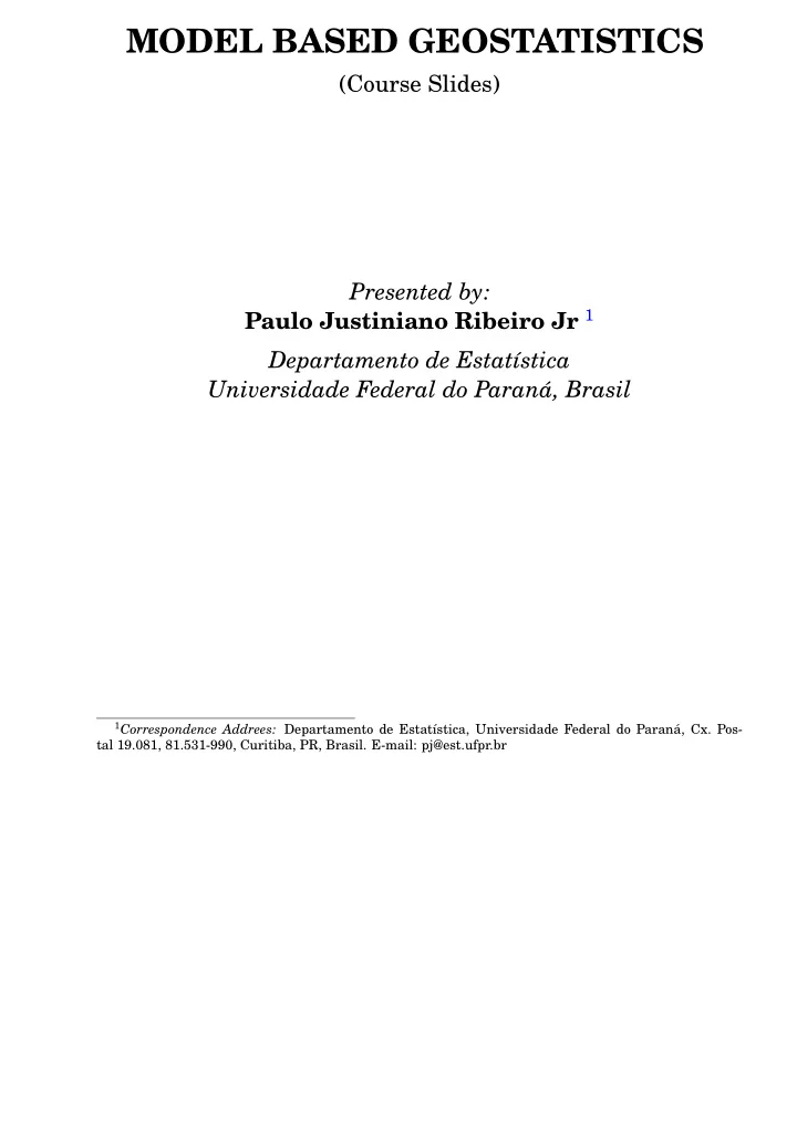
SLIDE 70

all data – “leaving-one-out”

100 300 500 100 300 500 data predicted + xx ++ xx x x+ + + x x + ++ x x x x + x xx x + + x + + x + x x x+ + + + + + + + + x ++ x + x x + + + x x x x x x + + + + + x x x + + x + x + x x + + x x + x x x x + + x + x x x + x + + + x x + x + x x + + + x x + + + x x + x + x + x x xx + x + x + x + + x x x x + x x x + + + x x x + ++ x x + x x x+ + x + x + x x x + x x x + x + x x x x + + x x + + x x + x x + + + + x + + x x x x x + x x x + x x + x + x x + + x + + + + + + x x + + x + + + + + + x x x + x + x + + x + x x x + + x x x + + x x + + + x + + x+ x + x x x + x x x x x x x x + + x + x + + + + + + x + x + x x x + + x x x x + + + x + + x x x x x x x x x x x + x + x + + + x + x + + x + + x + + + x x x + x + x x x + + + x x x + + + x + + + + x x x x + x + + + x + x +++ x x + + + ++ + x + x x x x + + + + x x + x x x x + x + x + x + + + x x + x + x x x x + + + + + x x x + + x + + x + + x x x x + x + x + + x x + + + x x x x x + x x x x x + x + + + x x x x 50 150 250 350 −50 50 150 250 Coord X Coord Y

+ + x x x x x + x x + + x + x x x + x + x + + x + + + + x x + + x x + x + x x x + x + x x + + x + + + x + + x + + + + x x + x x + x x x x x x x + x x x x x + + + x x x x x x x + + x + + x + + + + + + x x + + x x x x xx x + + + x x + + x x x + + x x x + x + x + + + x x + + x + x + + x + + + + + + x + x + x x x + + x x + x + x + x x x x + x x x x + + x x + x + x x + x + x x + + x x x x + + + x + x + x x x x + + x + x + + x x + x x x x

x x x x + x + x x + x + x + + + + x x + x x + x x + + x x x x + + + + + + x x x x x x x x + x + + x x + + + x x x x + x x + + x + x x x + + + + + + + x x x + + x x x x + + x x+ x + + + x + + x x + x + x x x x + + x x x + x x x + + + + x x x + + + + x + x + + + + + + + + + x x

x x + x x + x + + + x x + + + x x x x x + x + + x + + + x x + x x x x x + x x x x x + x + x x + x + + + + + x x x + x x x + +

+ x + + + + + x + + + x + + + x + + + + x + + x x

x + x x x + x + x + x +

+ +

x x

x +

+ +

x

data − predicted Density −200 −100 100 200 0.000 0.004 0.008 100 200 300 400 −200 100 200 predicted data − predicted + x x + + x x xx + + + x x ++ + x x x x + x x x x + + x + +x + x x x + ++ + + + + + + x + + x + x x + + + x x xx x x + + + + + x x x + + x + x + x x + + x x + x x x x + + x + x x x + x + + + x x + x + x x + + + x x + + + x x + x + x + x x x x + x + x + x + + x x x x + x x x + + + x x x + + + x x + x x x + + x + x + x x x + x xx + x + x x x x + + x x + + x x + x x + + + + x + + x x x x x + x x x + x x + x + x x + + x + + + + + + x x + + x + + + + + + x x x + x + x + + x + x x x + + x x x + + x x + + + x + + x + x + x x x + x x x x x x x x + + x + x + + + + + + x + x + x x x + + x x x x + + + x + + x x x x x x x x x x x + x + x + + + x + x + + x + + x + + + x x x + x + x x x + + + x x x + + + x + + + + x x x x + x + + + x + x ++ + x x + + + + + + x + x x x x + + + + x x + x x x x + x + x + x + + + x x + x + x x x x + + + + + x x x + + x + + x + + x x x x + x + x + + x x + + + x x x x x + x x x x x + x + + + x x x x 100 200 300 400 500 600 −200 100 200 data data − predicted + x x + + x xx x + + + x x+ + + x x xx + x x x x + + x + + x + x x x + + + + + + + + + x + + x + x x + + + x x x x x x + + + + + x x x + + x +x + x x + + x x + x x x x + + x + x x x + x + + + x x + x + x x + + + x x + + + x x + x + x + x x x x + x + x + x + + x x x x + x x x + + + x x x + + + x x + x x x + + x + x + x x x + x x x + x + x x x x + + x x + + x x + x x + + + + x + + x x x x x + x x x + x x + x + x x + + x + + + + + + x x + + x + + + + + + x x x + x + x + + x + x x x + + x x x + + x x + + + x + + x + x + x x x + x x x x x x x x + + x + x + + + + + + x + x + x x x + + x x x x + + + x + + x x x x xx x x x x x + x+ x + + + x + x + + x + + x + + + x x x + x + x x x + + + x x x + + + x + + + + x x x x + x + + + x + x + + + x x + + + + + + x + x x x x + + + + x x + x x x x + x + x + x + + + x x + x + x x x x + + + + + x x x + + x + + x + + x x x x + x + x + + x x + + + x x x x x + x x x x x + x + + + x x x x 0.0 0.2 0.4 0.6 0.8 1.0 0.0 0.2 0.4 0.6 0.8 1.0 theoretical prob

bserved prob

50 150 250 350 −50 50 150 250 Coord X Coord Y

x + + x x x + x x x + + + x + + + x x x x x x x + + + + + x x + + x x + + x x + x x + x + + + + x + + + + + x x x x + + x x x + + x + x x + x + x x + + x + x x x x x x + x x x + x + + + x + x x + x + + + + x + + + x + x + x x x + x + x + + + + x x + + + x x x x + x x + x + + x x x + x x + x + x x + + + x + + + + + + + + x

+ x + x + + + x x x x x + + x x x x x x + + x + + x x x x x x x x x + x x x + + x + x x + x x + x + + + + + x x + x + x + x + + + x + + x x + + + x x + x x + x x + x x x x x x x x x + x x + x x + + + x x x + + + x x + x + + x x + x + + + x + + x + x + x x x + x x + + x x + x + x x + x

+ x + x x x x x x x x x + x x x x + + x x x + x + x x x x + + + + x x x x x + x + x x x + x x x x x x + x + + + x x + x + x + x + + + + x x + x + x + + + x + x + x x

x + + + + + x x + + + + + + x + + + x x x x + x x + x x x x + + + x + + + +

x + x x + x x x + + + + + + + x+ + + + + x + x + x

+ x x x x

+ x x + + +

+ +

x

+

std error Density −4 −2 2 4 0.0 0.1 0.2 0.3 0.4 100 200 300 400 −4 −2 2 4 predicted std error + x x + + x x xx + + + x x ++ + x x x x + x x x x + + x + + x + x x x + ++ + + + + + + x + + x + x x + + + x x xx x x + + + + + x x x + + x + x + x x + + x x + x x x x + + x + x x x + x + + + x x + x + x x + + + x x + + + x x + x + x + x x x x + x + x + x + + x x x x + x x x + + + x x x + + + x x + x x x + + x + x + x x x + x xx + x + x x x x + + x x + + x x + x x + + + + x + + x x x x x + x x x + x x + x + x x + + x + + + + + + x x + + x + + + + + + x x x + x + x + + x + x x x + + x x x + + x x + + + x + + x + x + x x x + x x x x x x x x + + x + x + + + + + + x + x + x x x + + x x x x + + + x + + x x x x x x x x x x x + x + x + + + x + x + + x + + x + + + x x x + x + x x x + + + x x x + + + x + + + + x x x x + x + + + x + x ++ + x x + + + + + + x + x x x x + + + + x x + x x x x + x + x + x + + + x x + x + x x x x + + + + + x x x + + x + + x + + x x x x + x + x + + x x + + + x x x x x + x x x x x + x + + + x x x x 100 200 300 400 500 600 −4 −2 2 4 data std error + x x + + x xx x + + + x x + + + x x xx + x x x x + + x + + x + x x x + + + + + + + + + x + + x + x x + + + x x x x x x + + + + + x x x + + x +x + x x + + x x + x x x x + + x + x x x + x + + + x x + x + x x + + + x x + + + x x + x + x + x x x x + x + x + x + + x x x x + x x x + + + x x x + + + x x + x x x + + x + x + x x x + x x x + x + x x x x + + x x + + x x + x x + + + + x + + x x x x x + x x x + x x + x + x x + + x + + + + + + x x + + x + + + + + + x x x + x + x + + x + x x x + + x x x + + x x + + + x + + x + x + x x x + x x x x x x x x + + x + x + + + + + + x + x + x x x + + x x x x + + + x + + x x x x xx x x x x x + x+ x + + + x + x + + x + + x + + + x x x + x + x x x + + + x x x + + + x + + + + x x x x + x + + + x + x + + + x x + + + + + + x + x x x x + + + + x x + x x x x + x + x + x + + + x x + x + x x x x + + + + + x x x + + x + + x + + x x x x + x + x + + x x + + + x x x x x + x x x x x + x + + + x x x x

68

SLIDE 71

PART IV: BAYESIAN INFERENCE FOR THE GAUSSIAN MODEL

1. Basic Concepts
2. Bayesian Analysis of the Gaussian Model
3. A Case Study: Swiss Rainfall data

69

SLIDE 72

1. Bayesian Analysis - Basic Concepts

Bayesian inference deals with parameter uncer- tainty by treating parameters as random vari- ables, and expressing inferences about parame- ters in terms of their conditional distributions, given all observed data. For inference about model parameters, the full model specification now should include the mo- del parameters: [Y, θ] = [θ][Y |θ] Bayes’ Theorem allows us to calculate: [Y, θ] = [Y |θ][θ] = [Y ][θ|Y ] Thus, [θ|Y ] = [Y |θ][θ]/[Y ] is the posterior distribution where [Y ] =

[Y |θ][θ]dθ.

70

SLIDE 73

The Bayesian paradigm: (a) Model

the full model specification consists of

[Y, θ] = [Y |θ][θ].

formulate a model for the observable vari-

able Y .

this model defines [Y |θ] (and hence an ex-

pression for the log-likelihood ℓ(θ; Y )) (b) Prior

before we observe Y , the marginal [θ] ex-

presses our uncertainty about θ

call [θ] prior distribution for θ

(c) Posterior

having observed Y , it is no longer an unk-

nown (randomly varying) quantity

therefore revise uncertainty about θ by

conditioning on the observed value of Y

call [θ|Y ] posterior distribution for θ, and

use it to make inferential statements NOTE: the likelihood function occupies a cen- tral role in both classical and Bayesian infe- rence

71

SLIDE 74

Example: Swiss rainfall data

50 100 150 200 20 40 60 80 100 distance semivariance WLS ML posterior mode

Fitted variograms (100 data), using three different methods of estimation: (a) curve-fitting (thin line); (b) ML (dashed line); (c) posterior mode (thick line).

72

SLIDE 75

Prediction Because Bayesian inference treats θ as a ran- dom variable, it makes no formal distinction between parameter estimation problems and prediction problems, and thereby provides a na- tural means of allowing for parameter uncer- tainty in predictive inference. The general idea for prediction is to formulate a model for [Y, T, θ] = [Y, T|θ][θ] and make inferences based on the conditional distribution [T|Y ] =

[T, θ|Y ]dθ

=

[θ|Y ][T|Y, θ]dθ

73

SLIDE 76

Comparing plug-in and Bayesian

the plug-in prediction corresponds to inferen-

ces about [T|Y, ˆ θ]

Bayesian prediction is a weighted average of

plug-in predictions, with different plug-in va- lues of θ weighted according to their conditi-

nal probabilities given the observed data.

Bayesian prediction is usually more cautious than plug-in prediction, or in other words:

allowance for parameter uncertainty usually

results in wider prediction intervals Notes: (a) Until recently, the need to evaluate the in- tegral which defines [Y ] represented a major

bstacle to practical application.

(b) Development of Markov Chain Monte Carlo (MCMC) methods has transformed the situa- tion. (c) BUT, for geostatistical problems, reliable implementation of MCMC is not straight- forward. Geostatistical models don’t have a natural Markovian structure for the algo- rithms work well. (d) in particular for the Gaussian model other al- gorithms can be implemented.

74

SLIDE 77

2. Results for the Gaussian Model

Uncertainty only in the mean parameter Assume for now that only the mean parameter β is regarded as random with (conjugate) prior: β ∼ N

mβ ; σ2Vβ
The posterior is given by

[β|Y ] ∼ N((V −1

β

+ F ′R−1F)−1(V −1

β mβ + F ′R−1y) ;

σ2 (V −1

β

+ F ′R−1F)−1) ∼ N

ˆ

β ; σ2 Vˆ

β

The predictive distribution is

p(S∗|Y, σ2, φ) =

p(S∗|Y, β, σ2, φ) p(β|Y, σ2, φ) dβ.

with mean and variance given by

E[S∗|Y ] = (F0 − r′V −1F)(V −1

β

+ F ′V −1F)−1V −1

β mβ +

r′V −1 + (F0 − r′V −1F)(V −1

β

+ F ′V −1F)−1F ′V −1 Y Var[S∗|Y ] = σ2 V0 − r′V −1r+ (F0 − r′V −1F)(V −1

β

+ F ′V −1F)−1(F0 − r′V −1F)′ .

The predictive variance has three interpreta- ble components: a priori variance, the reduc- tion due to the data and the uncertainty in the mean. Vβ → ∞ corresponds to universal (or ordinary) kriging.

75

SLIDE 78

Uncertainty for all model parameters Assume (w.l.g.) a model without measurement error and the prior p(β, σ2, φ) ∝ 1

σ2p(φ).

The posterior distribution: p(β, σ2, φ|y) = p(β, σ2|y, φ) p(φ|y) pr(φ|y) ∝ pr(φ) |Vˆ

β|

1 2 |Ry|−1 2 (S2)−n−p 2 .

Algorithm 1: (a) Discretise the distribution [φ|y], i.e. choose a range of values for φ which is sensible for the particular application, and assign a discrete uniform prior for φ on a set of values span- ning the chosen range. (b) Compute the posterior probabilities on this discrete support set, defining a discrete posterior distribution with probability mass function ˜ pr(φ|y), say. (c) Sample a value of φ from the discrete distri- bution ˜ pr(φ|y). (d) Attach the sampled value of φ to the distribu- tion [β, σ2|y, φ] and sample from this distribu- tion. (e) Repeat steps (3) and (4) as many times as required; the resulting sample of triplets (β, σ2, φ) is a sample from the joint posterior distribution.

76

SLIDE 79

The predictive distribution is given by: p(S∗|Y ) = p(S∗, β, σ2, φ|Y ) dβ dσ2 dφ = p

s∗, β, σ2|y, φ
dβ dσ2 pr(φ|y) dφ

=

p(S∗|Y, φ) p(φ|y) dφ.

To sample from this distribution: Algorithm 2: (a) Discretise [φ|Y ], as in Algorithm 1. (b) Compute the posterior probabilities on the discrete support set. Denote the resulting distribution ˜ pr(φ|y). (c) Sample a value of φ from ˜ pr(φ|y). (d) Attach the sampled value of φ to [s∗|y, φ] and sample from it obtaining realisations of the predictive distribution. (e) Repeat steps (3) and (4) as many times as re- quired to generate a sample from the requi- red predictive distribution.

77

SLIDE 80

Note: (a) The algorithms are of the same kind to treat τ and/or κ as unknown parameters. (b) We specify a discrete prior distribution on a multi-dimensional grid of values. (c) This implies extra computational load (but no new principles)

78

SLIDE 81

3. A Case Study:

Swiss rainfall, 100 data

60 80 120 −563.5 −562.5 σ2 profile log−likelihood 15 20 25 −563.5 −562.5 φ profile log−likelihood

Profile likelihoods for covariance parameters: σ2; φ

σ2 Density 200 400 600 800 0.000 0.005 0.010 0.015 φ Density 20 40 60 80 100 0.00 0.05 0.10 0.15

Posterior distributions for covariance parameters: σ2; φ

σ2 φ 50 100 150 200 10 15 20 25 30 35 200 400 600 800 10 20 30 40 50 60 70 80 σ2 φ

2D profile log-likelihood (left) and samples from posterior distributions (right) for parameters σ2 and φ

79

SLIDE 82

Swiss rainfall: prediction results

50 100 150 200 250 300 350 −50 50 100 150 200 250 Coords X Coords Y

7 150 294 437 581

50 100 150 200 250 300 350 −50 50 100 150 200 250 Coords X Coords Y

8 5297 10587 15876 21165

Predicted signal surfaces and associated measures of pre- cision for the rainfall data: (a) posterior mean; (b) poste- rior variance

50 100 150 200 250 300 350 −50 50 100 150 200 250 Coords X Coords Y

0.1 0.5 0.9 1

Posterior probability contours for levels 0.10, 0.50 and 0.90 for the random set T = {x : S(x) < 150}

80

SLIDE 83

Swiss rainfall: prediction results (cont.)

50 100 150 200 250 300 350 −50 50 100 150 200 250 Coords X Coords Y 1 2 3 4

Recording stations and selected prediction locations (1 to 4)

100 200 300 400 500 600 0.000 0.005 0.010 0.015 rainfall density

Loc. 1
Loc. 2
Loc. 3
Loc. 4

Bayesian predictive distributions for average rainfall at selected locations.

81

SLIDE 84

Comments

nugget effect
other covariates (altitude, temperature, etc)
data “peculiarities”
(variogram) estimation: REML vs Bayesian
priors
Bayesian implementation algorithm
spatial-temporal modelling
vector random fields
ad hoc vs(?) model-based

82

SLIDE 85

PART V: GENERALIZED LINEAR SPATIAL MODELS

1. Generalized linear mixed models
2. Inference for the generalized linear geostatistical

model

3. Application of MCMC to Generalized Linear Pre-

diction

4. Case-study: Rongelap Island
5. Case-study: Gambia Malaria

SLIDE 86

Non-Gaussian data

Positive data:

1 2 3 4 5 0.0 0.3 0.6

Count data:

1 2 3 4 5 6 7 0.00 0.15 0.30

Binomial data:

1 2 3 4 0.00 0.15 0.30

Positive data with zeros:

0.0 0.3 0.6 84

SLIDE 87

Towards a model specification

The linear model Y = Fβ + ε can be written as: Yi ∼ N(µi, σ2) µi = k

j=1 fijβj

and generalized in two ways Yi ∼ Q(µ, ...) h(µi) = k

j=1 fijβj,

where Q is distribution in the exponential fa- mily and h(·): known link function

Generalized Linear Models (GLM)
no longer requires: normality, homocedasticity,

continuous scale

linear model: particular case

85

SLIDE 88

Generalized Linear Mixed Models

Classical generalized linear model has

Yi : i = 1, ..., n

mutually independent, with µi = E[Yi]

h(µi) = k

j=1 fijβj,

for known link function h(·) Generalized linear mixed model has

Yi : i = 1, ..., n

mutually independent, with µi = E[Yi], conditio- nal on realised values of a set of latent random variables Ui

h(µi) = Ui + k

j=1 fijβj,

for known link function h(·) Generalized linear geostatistical model has

Yi : i = 1, ..., n

mutually independent, with µi = E[Yi], conditio- nal on realised values of a set of latent random variables Ui

h(µi) = Ui + p

j=1 fijβj,

for known link function h(·)

Ui = S(xi)

where {S(x) : x ∈ I R2} is a spatial stochastic process

86

SLIDE 89

Examples

x1, . . . , xn locations with observations Poisson-log

[Y (xi) | S(xi)] is Poisson with density

f(z; µ) = exp(−µ)µz/z! z = 0, 1, 2, . . .

link: E[Y (xi) | S(xi)] = µi = exp(S(xi))

Binomial-logit

[Y (xi) | S(xi)] is binomial with density

f(z; µ) = r z

(µ/r)z(1 − µ/r)r−µ z = 0, 1, . . . , r
link: µi = E[Y (xi) | S(xi)] , S(xi) = log(µi/(r − µi))

Likelihood function

L(θ) =

I

R

n

i

f(yi; h−1(si))f(s | θ)ds1, . . . , dsn High-dimensional integral !!!

87

SLIDE 90

Inference For The Generalized Linear Geostatistical Model

likelihood evaluation involves high-dimensional

numerical integration

approximate methods (eg Breslow and Clayton,

1993) are of uncertain accuracy

MCMC is feasible, although not routine.

88

SLIDE 91

Application of MCMC to Generalized Linear Prediction

Ingredients

· Prior distributions for regression parameters β and covariance parameters θ · Data: Y = (Y1, ..., Yn) · S = (S(x1), ..., S(xn)) · S∗ = all other S(x)

Conditional independence structure

Y S θ S*

Use output from chain to construct posterior

probability statements about [T|Y ], where T = F(S∗)

89

SLIDE 92

Case-study: Rongelap Island

This case-study illustrates a model-based geosta- tistical analysis combining:

a Poisson log-linear model for the sampling dis-

tribution of the observations, conditional on a latent Gaussian process which represents spatial vari- ation in the level of contamination

Bayesian prediction of non-linear functionals of

the latent process

MCMC implementation

Details are in Diggle, Moyeed and Tawn (1998).

90

SLIDE 93

Radiological survey of Rongelap Island

Rongelap Island

– approximately 2500 miles south-west

f

Hawaii – contaminated by nuclear weapons testing du- ring 1950’s – evacuated in 1985 – now safe for re-settlement?

The statistical problem

– field-survey of 137Cs measurements – estimate spatial variation in 137Cs radioacti- vity – compare with agreed safe limits

91

SLIDE 94

Poisson Model for Rongelap Data

Basic measurements are nett counts Yi over

time-intervals ti at locations xi (i = 1, ..., n)

Suggests following model:

· S(x) : x ∈ R2 stationary Gaussian process (local radioactivity) · Yi|{S(·)} ∼ Poisson(µi) · µi = tiλ(xi) = ti exp{S(xi)}.

Aims:

· predict λ(x) over whole island · max λ(x) · arg(max λ(x))

92

SLIDE 95

Predicted radioactivity surface using log- Gaussian kriging

6000
5000
4000
3000
2000
1000
5000
4000
3000
2000
1000

1000 2 4 6 8 10

93

SLIDE 96

Predicted radioactivity surface using Pois- son log-linear model with latent Gaussian process

6000
5000
4000
3000
2000
1000
5000
4000
3000
2000
1000

1000 5 10 15

The

two maps above show the difference between: – log-Gaussian kriging of observed counts per unit time – log-linear analysis of observed counts

the principal visual difference is in the extent
f spatial smoothing of the data, which in turn

stems from the different treatments of the nug- get variance

94

SLIDE 97

Bayesian prediction of non-linear functio- nals of the radioactivity surface The left-hand panel shows the predictive distribu- tion of maximum radioactivity, contrasting the ef- fects of allowing for (solid line) or ignoring (dotted line) parameter uncertainty; the right-hand panel shows 95% pointwise credible intervals for the pro- portion of the island over which radioactivity exce- eds a given threshold.

Intensity level Density 10 20 30 40 50 60 0.0 0.02 0.04 0.06 0.08 0.10 0.12 0.14 Intensity level Survivor function 5 10 15 20 0.0 0.2 0.4 0.6 0.8 1.0 5 10 15 20 0.0 0.2 0.4 0.6 0.8 1.0 5 10 15 20 0.0 0.2 0.4 0.6 0.8 1.0

95

SLIDE 98

The two panels of the above diagram illustrate

Bayesian prediction of non-linear functionals of the latent Gaussian process in the Poisson log-linear mo- del

the left-hand panel contrasts posterior distribu-

tions of the maximum radioactivity based on: (i) the fully Bayesian analysis incorporating the effects of parameter uncertainty in addition to uncertainty in the latent process (solid line) (ii) fixing the model parameters at their estima- ted values, ie allowing for uncertainty only in the latent process

the right-hand panel gives posterior estimates

with 95% point-wise credible intervals for the proportion of the island over which radioactivity exceeds a given threshold (dotted line).

96

SLIDE 99

Case-study: Gambia malaria

In this example, the spatial variation is of se-

condary scientific importance.

The primary scientific interest is to describe

how the prevalence of malarial parasites de- pends on explanatory variables measured: – on villages – on individual children

There is a particular scientific interest in

whether a vegetation index derived from satel- lite data is a useful predictor of malaria preva- lence, as this would help health workers to de- cide how to make best use of scarce resources.

97

SLIDE 100

Data-structure

2039 children in 65 villages
test each child for presence/absence of malaria

parasites Covariate information at child level:

age (days)
sex (F/M)
use of mosquito net (none, untreated, treated)

Covariate information at village level:

location
vegetation index, from satellite data
presence/absence of public health centre

98

SLIDE 101

Logistic regression model Logistic model for presence/absence in each child:

Yij = 0/1 for absence/presence of malaria para-

sites in jth child in ith village

fij = child-specific covariates
wi = village-specific covariate
logitP(Yij = 1|S(·)) = f ′

ijβ1 + wi′β2 + S(xi)

Is it reasonable to assume conditionally indepen- dent infections within same village? If not, we might wish to extend the model to allow for non-spatial extra-binomial variation:

Ui ∼ N(0, ν2)
logitP(Yij = 1|S(·), U) = f ′

ijβ1 + wi′β2 + Ui + S(xi)

99

SLIDE 102

Exploratory analysis

fit standard logistic linear model, ignoring S(x)

and/or U

compute for each village:

Ni = ni

j=1 Yij

µi = ni

j=1 ˆ

Pij σ2

i = ni j=1 ˆ

Pij(1 − ˆ Pij)

compute village-residuals, ri = (Ni − µi)/σi
apply conventional geostatistics to derived data

ri

variogram indicates residual spatial structure

100

SLIDE 103

Variogram of residuals

5 10 15 20 25 30 1 2 3 4 distance (km) semi−variance

101

SLIDE 104

Model-based geostatistical analysis α = intercept term in linear predictor β1 = regression coefficient for age β2 = regression coefficient for bed-net use β3 = regression coefficient for treated bed-net β4 = regression coefficient for green-ness index β5 = regression coefficient for presence of public he- alth centre in village ν2 = variance of non-spatial random effects Ui σ2 = variance of spatial process S(x) φ = rate of decay of spatial correlation with dis- tance κ = shape parameter for Mat´ ern correlation func- tion Param. 2.5% Qt. 97.5% Qt. Mean Median α

4.232073

1.114734

1.664353 -1.696228

β1 0.000442 0.000918 0.000677 0.000676 β2

0.684407
0.083811
0.383750 -0.385772

β3

0.778149

0.054543

0.355655 -0.355632

β4

0.039706

0.071505 0.018833 0.020079 β5

0.791741

0.180737

0.324738 -0.322760

ν2 0.000002 0.515847 0.117876 0.018630 σ2 0.240826 1.662284 0.793031 0.740790 φ 1.242164 53.351207 11.653717 7.032258 κ 0.150735 1.955524 0.935064 0.830548

note concentration of posterior for ν2 close to

zero

102

SLIDE 105

Map of the predicted surface ˆ S(x) (posterior mean)

Kilometres Kilometres 300 400 500 600 1400 1500 1600

1.5

0.0 1.0 Western Eastern 300 400 500 600 1400 1500 1600 300 400 500 600 1400 1500 1600 Central 300 400 500 600 1400 1500 1600

103

SLIDE 106

Posterior density estimates for S(x) at two se- lected locations.

S(x) Density

4
2

2 4 0.0 0.2 0.4 0.6 0.8 S(x) Density

4
2

2 4 0.0 0.2 0.4 0.6 0.8

x = (452, 1493) x = (520, 1497)

solid curve – remote location (452, 1493),
dashed curve – location (520, 1497), close to ob-

served sites in central region.

104

SLIDE 107

Empirical posterior distributions for regres- sion parameters

0.0004 0.0008 500 1000 1500 2000 2500 3000 beta_1 Density

1.0
0.6
0.2

0.2 0.0 0.5 1.0 1.5 2.0 beta_2 Density

1.0
0.5

0.0 0.0 0.5 1.0 1.5 beta_3 Density

o
o
o
o
o
o o
o
o
o
o
o
o
o
o
o
o
o
o
o
o
o
o
o
o
o
o
o
o
oo
o
o
o
o
o
o
o o
o
o
o o
o
o
o
o
o
o
o
o
o
o
o
oo
o
o
o
o
o
o
o
o
o
o
o
o
o
o
o o
o
o
o
o
o
o
o
o
o
o
o
o
o
o
o
o
o
o
o
o
o
o
o
o
o
o
o
o
o
o
o
o
o
o
o
o
oo
o
o
o
o
o
o
o
o
o
o
o
o
o
o
o
o
o
oo
o
o
o
o
o
o
o
o
beta_2

beta_3

1.0
0.6
0.2

0.2

1.0
0.5

0.0

β1 = effect of age
β2 = effect of untreated bed-nets
β3 = additional effect of treated bed-nets

105

SLIDE 108

Goodness-of-fit for Gambia malaria model

Fitted value

Residual 0.25 0.30 0.35 0.40 0.45 0.50 0.55

4
2

2 4

Village-level residuals against fitted values.

rij = (Yij − ˆ

pij)/√{ˆ pij(1 − ˆ pij)}

ri = rij/√ni
intended to check adequacy of model for pij

106

SLIDE 109

Distance (km) Variogram 10 20 30 40 50 60 0.5 1.0 1.5 2.0 2.5

Standardised residual empirical variogram plot (village-level data and pointwise 95% posterior intervals constructed from simulated realisations of fitted model).

rij = (Yij − ˆ

p∗

ij)/√{ˆ

p∗

ij(1 − ˆ

p∗

ij)}

ri = rij/√ni
logitp∗

ij = ˆ

α + f ′

ij ˆ

β + ˆ S(xi)

intended to check adequacy of model for S(x)

107

SLIDE 110

Is a geostatistical model necessary?

E[S(x)|data]

E[U|data]

2
1

1 2

2
1

1 2

Plot of estimated posterior means of random effects ˆ Ui from non-spatial GLMM against estimated posterior means ˆ S(xi) at observed locations in geostatistical model.

high correlation represents strong empirical

evidence of spatial dependence

but explicit modelling of spatial dependence has

small effect on inferences about regression pa- rameters

108

SLIDE 111

Generalised linear Spatial Models

Diggle, Tawn and Moyeed (1998). Error distribution [Y (x) | S(x)] Link function E[Y (x) | S(x)] = h−1(S(x)) Gaussian random field {S(x) : x ∈ A}

E[S(x)] = d(x)Tβ
Cov (S(x), S(x′)) = σ2ρ(x − x′; φ) + τ 21{x=x′}.

Structure:

Y S θ S*

Data : Y = (Y (x1), ..., Y (xn))
S = (S(x1), ..., S(xn))
S∗ = some other S(x)
θ parameters

109

SLIDE 112

Prediction with known parameters

From figure, prediction is separated into three steps.

Simulate

s(1), . . . , s(m) from [S|y] (using MCMC).

Simulate s∗(j) from [S∗|s(j)], j = 1, . . . , m

(multivariate Gaussian)

Approximate E[T(S∗)|y] by

1 m

m

j=0

T(s∗(j)) If possible: instead calculate E[T(S∗)|s(j)], j = 1, . . . , m directly, and estimate E[T(S∗)|y] by 1 m

m

j=0

E[T(S∗)|s(j)] Advantage: smaller Monte Carlo error

110

SLIDE 113

MCMC for conditional simulation

Let S = DTβ + Σ1/2Γ, Γ ∼ Nn(0, I). Conditional density of [Γ |Y = y] f(γ|y) ∝ f(y|γ)f(γ) Langevin-Hastings algorithm Proposal: γ′ from a Nn(ξ(γ), hI) where ξ(γ) = γ +

h 2∇ log f(γ | y).

Poisson-log Spatial model: ∇ log f(γ|y) = −γ + (Σ1/2)T(y − exp(s)) where s = Σ1/2γ. Expression generalises to other generalised linear spatial models. MCMCM output γ1, . . . , γm. Multiply by Σ1/2 and

btain: s(1), . . . , s(m) from [S|y].

111

SLIDE 114

Random walk Metropolis algorithm

Current state: γ.
Proposal: γ′ from a Nn(γ, hI).
Accept: γ′ with probability

a(γ, γ′) = 1 ∧ π(γ′) π(γ) .

Langevin-Hastings algorithm

Current state: γ.
Proposal: γ′ from a Nn(ξ(γ), hI) where

ξ(γ) = γ + h

2∇ log π(γ).

Accept: γ′ with probability

a(γ, γ′) = 1 ∧ π(γ′)q(γ′, γ) π(γ)q(γ, γ′) . Models considered here: ∇ log f(γ|y) = −γ+(Σ1/2)T

(yi − g−1(si))gc(g−1(si))

g(g−1(si)) n

i=1

. where s = Dβ + Σ1/2γ.

112

SLIDE 115

Geometric Ergodicity

Convergence rate to equilibrium is geometrically fast. Geometrical ergodicity ⇒ Central Limit Theorem: √m   1 m

m

j=1

ψ(Γ(j)) − E[ψ(Γ)|y]   → N(0, σ2

ψ).

when ψ(·)2 ≤ V (·) Random walk Metropolis: Conditions (Jarner and Hansen, 2000): lim sup

µ→m1,m2

1 g′(µ)

1

µ − yi + g′′

c(µ)

g′

c(µ) − g′′(µ)

g′(µ)

< ∞,

lim sup

µ→m1,m2

yi − µ g(µ) g′

c(µ)

g′(µ) ≤ 0, imply geometric ergodicity, with V (γ) = f(γ|y)−1/2. Langevin-Hastings:(Robert and Tweedie,1996) Poisson-log model (∇(γ) = −γ + QT(y − exp(s))) not

geom. ergodic.

Truncated Langevin-Hastings ∇(γ)trunc = −γ + QTR(γ) where R(γ) is a bounded function. Geometrically ergodic with V (γ) = exp(tγ).

113

SLIDE 116

MCMC for Bayesian inference

Parameters in underlying Gaussian model: S ∼ MV N(DTβ, σ2κ(φ)). S = DTβ + σκ(φ)1/2Γ, Γ ∼ Nn(0, I). Metropolis-within-Gibbs algorithm:

Update Γ from [Γ|y, β, log(σ), log(φ)]

(Langevin-Hasting described earlier)

Update

β from [β|Γ, log(σ), log(φ)] (RW- Metropolis)

Update

log(σ) from [log(σ)|Γ, β, log(φ)] (RW- Metropolis)

Update

log(φ) from [log(φ)|Γ, β, log(σ)] (RW- Metropolis) Prediction:

Simulate (s(j), β(j), σ2(j), φ(j)), j = 1, . . . , m

(using MCMC)

Simulate s∗(j) from [S∗|s(j), β(j), σ2(j), φ(j)],

j = 1, . . . , m (multivariate Gaussian) Discrete prior for φ is an advantage (reduced com- puting time). Thinning not to store a large sample of high- dimensional quantities.

114

SLIDE 117

Marginalisation Integrating out β and σ2.

Conjugate priors: β | σ2 ∼ N

mb ; σ2Vb
1/σ2 ∼ 1

S2

c

χ2 (nc) [scaled-inverse-χ2(nc, S2

c)]

Marginalisation

Posterior distribution is f(s|y) = f(y|s)fI(s),

where fI is the marginalised density for S.

Marginalisation makes [S∗|S] a multivariate-t

distribution. Procedure:

Simulate

s(1), . . . , s(m) from [S|y] (using MCMC).

Simulate s∗(j) from [S∗|s(j)], j = 1, . . . , m

(multivariate-t distribution)

Approximate E[T(S∗)|y] by

1 m

m

j=0

T(s∗(j))

115

SLIDE 118

Parameter estimation for generalized linear spatial model

Methods
f

moments (empirical vario- gram/covariogram)

Approximate methods: pseudo-likelihood (accu-

racy unknown). Monte Carlo approximation to likelihood Geyer and Thompson, 1992 ; Geyer, 1994. Define ˜ f(y) = f(y | s) ˜ f(s) for some density ˜ f(s). L(θ) =

I

R

n f(y | s)f(s | θ)ds ∝

I

R

n

f(y | s)f(s | θ) f(y | s) ˜ f(s) ˜ f(s | y)ds = ˜ E[f(S | θ) ˜ f(S) | y where ˜ E[· | y] is expectation w.r.t ˜ f(s | y).

How to chose ˜

f(s) ? – Could chose ˜ f(s) = f(s | θ0) for some θ0. – Instead we use ˜ f(s) = fI(s | ψ0) for some ψ0, where θ = (β, σ2, ψ), and fI(s | ψ0) is the marginalised density fI(s | ψ0) = fI(s | β, σ2, ψ0)π(β, σ2)dβdσ2 (using conjugate prior

n (β, σ2)).
Very useful as exploratory tool; exploring other

correlation functions, anisotropy, etc.

116

SLIDE 119

Priors

S ∼ Nn(Dβ, σ2R(φ)) Non-informative priors:

π(σ2) ∝ 1/σ2 commonly used, but gives improper

posterior !

π(φ) must be proper.
Thesis gives conditions for proper posterior.

Conjugate priors: β | σ2 ∼ N

mb ; σ2Vb
1/σ2 ∼ 1

S2

σ

χ2 (nσ) [scaled-inverse-χ2(nσ, S2

σ)]

Marginalisation

Conditional

distribution becomes f(s|y) ∝ f(y|s)fI(s), where fI is the marginalised density of S.

Marginalisation makes [S∗|S] a multivariate-t

distribution. Computationally advantageous in MCMC- algorithm. Conjugate prior for φ ?

117

SLIDE 120

PART VI: Further topics and conclusions

1. Multivariate methods
2. Non-linear methods
3. Space-time models
4. Marked point processes
5. Closing remarks

SLIDE 121

Multivariate methods

within linear Gaussian setting, extension to

multivariate data is straightforward in princi- ple

but specification of a useful class of default

models for cross-covariance structure is not straightforward

detailed implementation should be problem-

specific: for example, – (Y1, Y2) qualitatively different, and measured at a common set of locations? – Y2 a low-cost surrogate for Y1 of primary inte- rest?

119

SLIDE 122

Non-linear methods

non-linear mean response µ(x) with Gaussian

errors – straightforward in principle Example: plume model for dispersal of pollu- tant

intrinsically non-linear systems specified by

system of stochastic differential equations – a challenging problem Example: soil conductivity/transmissivity

120

SLIDE 123

Space-time models

Emerging space-time data-sets are big, and

present severe computational challenges.

Specific models are best defined in context.
Some examples:
1. Calibration
f

radar reflectance against ground-truth rainfall intensity (Brown, Dig- gle, Lord and Young, 2001). (a) Yit : i = 1, ..., n – ground-truth log-rainfall intensity at small number of sites xi (b) U(x, t) : x ∈ A – log-radar reflectance mea- sured effectively continuously over a study region A (c) Empirical model, Yit = α + B(xi, t)U(xi, t) where B(x, t) is continuous space-time Gaussian process (d) Spatial prediction, ˆ Y (x, t) = ˆ α + ˆ B(x, t)U(x, t)

121

SLIDE 124

2. On-line disease surveillance (Brix and Dig-

gle, 2001) (a) Data give population density λ0(x) (appro- ximately), plus locations of daily incident cases (b) Model space-time point process of incident cases as Cox process: – Poisson process with intensity λ(x, t) = λ0(x) exp{α + Z(x, t)} – Space-time Gaussian process Z(x, t) mo- dels variation in disease risk – Interested in early detection of changes in the risk surface, λ(x, t)/λ(x, t−1) = exp{Z(x, t)−Z(x, t−1)}

122

SLIDE 125

Marked point processes

Definition: a joint probability model for a stochas- tic point process P, and an associated set of ran- dom variables, or marks, M Different possible structural assumptions:

[P, M] = [P][M]

The random field model – often assumed implicitly in geostatistical work.

[P, M] = [P|M][M]

Preferential sampling – sampling locations are determined by partial knowledge of the un- derlying mark process

Example. deliberate siting of air pollution mo-

nitors in badly polluted areas.

[P, M] = [P][M|P]

Often appropriate when the mark process is

nly

defined at the sampling locations.

Example. Presence/absence of disease amongst

individual members of a population. Implications of ignoring violations of the random field model are not well understood.

123

SLIDE 126

Closing remarks

all models are wrong, but some models are use-

ful

whatever model is adopted, inferential procedu-

res which respect general statistical principles are likely to out-perform ad hoc procedures

ignoring parameter uncertainty can seriously

prejudice nominal prediction intervals

the Bayesian paradigm gives a workable inte-

gration of parameter estimation and stochastic process prediction, but results can be sensitive to joint prior specifications.

the best models are developed by statisticians