Mixed models in R using the lme4 package Part 1: Introduction to R - - PDF document

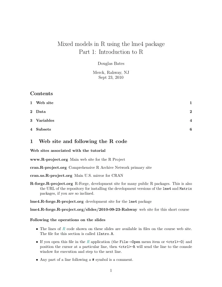
Mixed models in R using the lme4 package Part 1: Introduction to R

Douglas Bates Merck, Rahway, NJ Sept 23, 2010

Contents

1 Web site 1 2 Data 2 3 Variables 4 4 Subsets 6

1 Web site and following the R code

Web sites associated with the tutorial www.R-project.org Main web site for the R Project cran.R-project.org Comprehensive R Archive Network primary site cran.us.R-project.org Main U.S. mirror for CRAN R-forge.R-project.org R-Forge, development site for many public R packages. This is also the URL of the repository for installing the development versions of the lme4 and Matrix packages, if you are so inclined. lme4.R-forge.R-project.org development site for the lme4 package lme4.R-forge.R-project.org/slides/2010-09-23-Rahway web site for this short course Following the operations on the slides

• The lines of R code shown on these slides are available in files on the course web site.

The file for this section is called 1Intro.R.

• If you open this file in the R application (the File→Open menu item or <ctrl>-O) and

position the cursor at a particular line, then <ctrl>-R will send the line to the console window for execution and step to the next line.

• Any part of a line following a # symbol is a comment.

1

• The code is divided into named “chunks”, typically one chunk per slide that contains

code.

• In the system called Sweave used to generate the slides the result of a call to a graphics

function must be printed. In interactive use this is not necessary but neither is it harmful.

2 Organizing data

Organizing data in R

• Standard rectangular data sets (columns are variables, rows are observations) are stored

in R as data frames.

• The columns can be numeric variables (e.g. measurements or counts) or factor variables

(categorical data) or ordered factor variables. These types are called the class of the variable.

• The str function provides a concise description of the structure of a data set (or any
• ther class of object in R). The summary function summarizes each variable according to

its class. Both are highly recommended for routine use.

• Entering just the name of the data frame causes it to be printed. For large data frames

use the head and tail functions to view the first few or last few rows. Data input

• The simplest way to input a rectangular data set is to save it as a comma-separated value

(csv) file and read it with read.csv.

• The first argument to read.csv is the name of the file. On Windows it can be tricky

to get the file path correct (backslashes need to be doubled). The best approach is to use the function file.choose which brings up a “chooser” panel through which you can select a particular file. The idiom to remember is

> mydata <- read.csv(file.choose ())

for comma-separated value files or

> mydata <- read.delim(file.choose ())

for files with tab-delimited data fields.

• If you are connected to the Internet you can use a URL (within quotes) as the first

argument to read.csv or read.delim. (See question 1 in the first set of exercises) In-built data sets

• One of the packages attached by default to an R session is the datasets package that

contains several data sets culled primarily from introductory statistics texts.

• We will use some of these data sets for illustration.

2

• The Formaldehyde data are from a calibration experiment, Insectsprays are from an

experiment on the effectiveness of insecticides.

• Use ? followed by the name of a function or data set to view its documentation. If

the documentation contains an example section, you can execute it with the example function. The Formaldehyde data

> str(Formaldehyde) ’data.frame’: 6 obs. of 2 variables: $ carb : num 0.1 0.3 0.5 0.6 0.7 0.9 $ optden: num 0.086 0.269 0.446 0.538 0.626 0.782 > summary(Formaldehyde) carb

• ptden

Min. :0.1000 Min. :0.0860 1st Qu.:0.3500 1st Qu.:0.3132 Median :0.5500 Median :0.4920 Mean :0.5167 Mean :0.4578 3rd Qu.:0.6750 3rd Qu.:0.6040 Max. :0.9000 Max. :0.7820 > Formaldehyde carb optden 1 0.1 0.086 2 0.3 0.269 3 0.5 0.446 4 0.6 0.538 5 0.7 0.626 6 0.9 0.782

The InsectSprays data

> str(InsectSprays) ’data.frame’: 72 obs. of 2 variables: $ count: num 10 7 20 14 14 12 10 23 17 20 ... $ spray: Factor w/ 6 levels "A","B","C","D",..: 1 1 1 1 1 1 1 1 1 .. > summary(InsectSprays) count spray Min. : 0.00 A:12 1st Qu.: 3.00 B:12 Median : 7.00 C:12 Mean : 9.50 D:12 3rd Qu.:14.25 E:12 Max. :26.00 F:12

3

> head(InsectSprays) count spray 1 10 A 2 7 A 3 20 A 4 14 A 5 14 A 6 12 A

Copying, saving and restoring data objects

• Assigning a data object to a new name creates a copy.
• You can save a data object to a file, typically with the extension .rda or .Rdata, using

the save function.

• To restore the object you load the file.

> sprays <- InsectSprays > save(sprays , file = "sprays.rda") > rm(sprays) > ls.str() > load("sprays.rda") > names(sprays) [1] "count" "spray"

3 Accessing and modifying variables

Accessing and modifying variables

• The $ operator is used to access variables within a data frame.

> Formaldehyde$carb [1] 0.1 0.3 0.5 0.6 0.7 0.9

• You can also use $ to assign to a variable name

> sprays$sqrtcount <- sqrt(sprays$count) > names(sprays) [1] "count" "spray" "sqrtcount"

• Assigning the special value NULL to the name of a variable removes it.

> sprays$sqrtcount <- NULL > names(sprays) [1] "count" "spray"

4

Using with and within

• In complex expressions it can become tedious to repeatedly type the name of the data

frame.

• The with function allows for direct access to variable names within an expression. It

provides “read-only” access.

> Formaldehyde$carb * Formaldehyde$optden [1] 0.0086 0.0807 0.2230 0.3228 0.4382 0.7038 > with(Formaldehyde , carb * optden) [1] 0.0086 0.0807 0.2230 0.3228 0.4382 0.7038

• The within function provides read-write access to a data frame. It does not change the
• riginal frame; it returns a modified copy. To change the stored object you must assign

the result to the name.

> str(sprays <- within(sprays , sqrtcount <- sqrt(count ))) ’data.frame’: 72 obs. of 3 variables: $ count : num 10 7 20 14 14 12 10 23 17 20 ... $ spray : Factor w/ 6 levels "A","B","C","D",..: 1 1 1 1 1 1 1 .. $ sqrtcount: num 3.16 2.65 4.47 3.74 3.74 ...

Data Organization

• Careful consideration of the data layout for experimental or observational data is repaid

in later ease of analysis. Sadly, the widespread use of spreadsheets does not encourage such careful consideration.

• If you are organizing data in a table, use consistent data types within columns. Databases

require this; spreadsheets don’t.

• A common practice in some disciplines is to convert categorical data to 0/1 “indicator

variables” or to code the levels as numbers with a separate “data key”. This practice is unnecessary and error-inducing in R. When you see categorical variables coded as numeric variables, change them to factors or ordered factors.

• Spreadsheets also encourage the use of a “wide” data format, especially for longitudinal
• data. Each row corresponds to an experimental unit and multiple observation occasions

are represented in different columns. The “long” format is preferred in R. 5

Converting numeric variables to factors

• The factor (ordered) function creates a factor (ordered factor) from a vector. Factor

labels can be specified in the optional labels argument.

• Suppose the spray variable in the InsectSprays data was stored as numeric values

1, 2, . . . , 6. We convert it back to a factor with factor.

> str(sprays <- within(InsectSprays , spray <- as.integer(spray ))) ’data.frame’: 72 obs. of 2 variables: $ count: num 10 7 20 14 14 12 10 23 17 20 ... $ spray: int 1 1 1 1 1 1 1 1 1 1 ... > str(sprays <- within(sprays , spray <- factor(spray , + labels = LETTERS [1:6]))) ’data.frame’: 72 obs. of 2 variables: $ count: num 10 7 20 14 14 12 10 23 17 20 ... $ spray: Factor w/ 6 levels "A","B","C","D",..: 1 1 1 1 1 1 1 1 1 ..

4 Subsets of data frames

Subsets of data frames

• The subset function is used to extract a subset of the rows or of the columns or of both

from a data frame.

• The first argument is the name of the data frame. The second is an expression indicating

which rows are to be selected.

• This expression often uses logical operators such as ==, the equality comparison, or !=,

the inequality comparison, >=, meaning “greater than or equal to”, etc.

> str(sprayA <- subset(sprays , spray == "A")) ’data.frame’: 12 obs. of 2 variables: $ count: num 10 7 20 14 14 12 10 23 17 20 ... $ spray: Factor w/ 6 levels "A","B","C","D",..: 1 1 1 1 1 1 1 1 1 ..

• The optional argument select can be used to specify the variables to be included. There

is an example of its use in question 4 of the first set of exercises. 6

Subsets and factors

• The way that factors are defined, a subset of a factor retains the original set of levels.

Usually this is harmless but sometimes it can cause unexpected results.

• You can “drop unused levels” by applying factor to the factor. Many functions, such

as xtabs, which is used to create cross-tabulations, have optional arguments with names like drop.unused.levels to automate this.

> xtabs(~spray , sprayA) spray A B C D E F 12 > xtabs(~spray , sprayA , drop = TRUE) spray A 12

Dropping unused levels in the spray factor and %in%

> str(sprayA <- within(sprayA , spray <- factor(spray ))) ’data.frame’: 12 obs. of 2 variables: $ count: num 10 7 20 14 14 12 10 23 17 20 ... $ spray: Factor w/ 1 level "A": 1 1 1 1 1 1 1 1 1 1 ... > xtabs(~spray , sprayA) spray A 12

• Another useful comparison operator is %in% for selecting a subset of the values in a

variable.

> str(sprayDEF <- subset(sprays , spray %in% c("D", "E", + "F"))) ’data.frame’: 36 obs. of 2 variables: $ count: num 3 5 12 6 4 3 5 5 5 5 ... $ spray: Factor w/ 6 levels "A","B","C","D",..: 4 4 4 4 4 4 4 4 4 ..

7

“Long” and “wide” forms of data

• Spreadsheet users tend to store balanced data, such as InsectSprays, across many

columns. This is called the “wide” format. The unstack function converts a simple “long” data set to wide; stack for the other way.

> str(unstack(InsectSprays )) ’data.frame’: 12 obs. of 6 variables: $ A: num 10 7 20 14 14 12 10 23 17 20 ... $ B: num 11 17 21 11 16 14 17 17 19 21 ... $ C: num 0 1 7 2 3 1 2 1 3 0 ... $ D: num 3 5 12 6 4 3 5 5 5 5 ... $ E: num 3 5 3 5 3 6 1 1 3 2 ... $ F: num 11 9 15 22 15 16 13 10 26 26 ...

• The problem with the wide format is that it only works for balanced data. A designed

experiment may produce balanced data (although “Murphy’s Law” would indicate oth- erwise) but observational data are rarely balanced.

• Stay with the long format (all the observations on all the units are in a single column)

when possible. Using reshape

• The reshape function allows for more general translations of long to wide and vice-versa.

It is specifically intended for longitudinal data.

• There is also a package called "reshape" with even more general (but potentially con-

fusing) capabilities.

• Phil Spector’s book, Data Manipulation with R (Springer, 2008) covers this topic in more

detail. Determining unique rows in a data frame

• One disadvantage of keeping data in the long format is redundancy and the possibility
• f inconsistency.
• In the first set of exercises you are asked to create a data frame classroom from a csv file

available on the Internet. Each of the 1190 rows corresponds to a student in a classroom in a school. There is one numeric “school level” covariate, housepov.

• To check if housepov is stored consistently we select the unique combinations of only

those two columns

> str(unique(subset(classroom , select = c(schoolid , housepov )))) ’data.frame’: 107 obs. of 2 variables: $ schoolid: Factor w/ 107 levels "1","2","3","4",..: 1 2 3 4 5 6 7.. $ housepov: num 0.082 0.082 0.086 0.365 0.511 0.044 0.148 0.085 0..

Because there are 107 unique combinations and 107 schools, housepov is consistent with schoolid. 8

Summary

• Most common data organization is as a data.frame, which is a rectangular table. Columns

can be numeric, factors, ordered factors, dates, date/time values, etc.

• Data can be read from “flat files” either locally or over the web. Variables are accessed
• r modified using the $ operator or functions with() and within().
• The str(), summary() and subset() functions are versatile and worth learning.
• For longitudinal and other data, prefer the “long” format to the “wide” format.

9