Methods for handling uncertainty Default or nonmonotonic logic: - PDF document

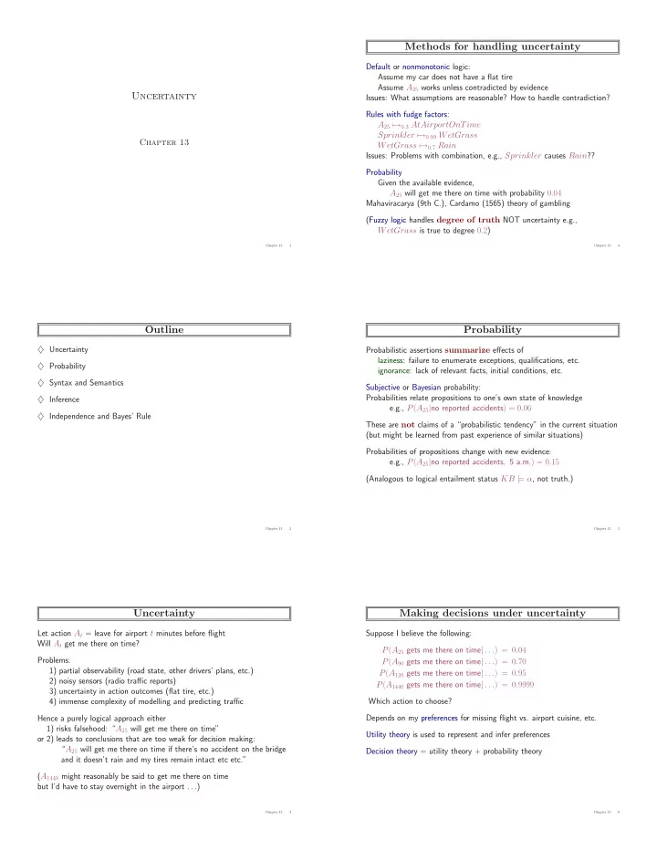
Methods for handling uncertainty Default or nonmonotonic logic: Assume my car does not have a flat tire Assume A 25 works unless contradicted by evidence Uncertainty Issues: What assumptions are reasonable? How to handle contradiction? Rules with fudge factors: A 25 �→ 0 . 3 AtAirportOnTime Sprinkler �→ 0 . 99 WetGrass Chapter 13 WetGrass �→ 0 . 7 Rain Issues: Problems with combination, e.g., Sprinkler causes Rain ?? Probability Given the available evidence, A 25 will get me there on time with probability 0 . 04 Mahaviracarya (9th C.), Cardamo (1565) theory of gambling (Fuzzy logic handles degree of truth NOT uncertainty e.g., WetGrass is true to degree 0 . 2 ) Chapter 13 1 Chapter 13 4 Outline Probability ♦ Uncertainty Probabilistic assertions summarize effects of laziness: failure to enumerate exceptions, qualifications, etc. ♦ Probability ignorance: lack of relevant facts, initial conditions, etc. ♦ Syntax and Semantics Subjective or Bayesian probability: Probabilities relate propositions to one’s own state of knowledge ♦ Inference e.g., P ( A 25 | no reported accidents ) = 0 . 06 ♦ Independence and Bayes’ Rule These are not claims of a “probabilistic tendency” in the current situation (but might be learned from past experience of similar situations) Probabilities of propositions change with new evidence: e.g., P ( A 25 | no reported accidents , 5 a.m. ) = 0 . 15 (Analogous to logical entailment status KB | = α , not truth.) Chapter 13 2 Chapter 13 5 Uncertainty Making decisions under uncertainty Let action A t = leave for airport t minutes before flight Suppose I believe the following: Will A t get me there on time? P ( A 25 gets me there on time | . . . ) = 0 . 04 Problems: P ( A 90 gets me there on time | . . . ) = 0 . 70 1) partial observability (road state, other drivers’ plans, etc.) P ( A 120 gets me there on time | . . . ) = 0 . 95 2) noisy sensors (radio traffic reports) P ( A 1440 gets me there on time | . . . ) = 0 . 9999 3) uncertainty in action outcomes (flat tire, etc.) 4) immense complexity of modelling and predicting traffic Which action to choose? Hence a purely logical approach either Depends on my preferences for missing flight vs. airport cuisine, etc. 1) risks falsehood: “ A 25 will get me there on time” Utility theory is used to represent and infer preferences or 2) leads to conclusions that are too weak for decision making: “ A 25 will get me there on time if there’s no accident on the bridge Decision theory = utility theory + probability theory and it doesn’t rain and my tires remain intact etc etc.” ( A 1440 might reasonably be said to get me there on time but I’d have to stay overnight in the airport . . . ) Chapter 13 3 Chapter 13 6

Probability basics Why use probability? Begin with a set Ω —the sample space The definitions imply that certain logically related events must have related e.g., 6 possible rolls of a die. probabilities ω ∈ Ω is a sample point/possible world/atomic event E.g., P ( a ∨ b ) = P ( a ) + P ( b ) − P ( a ∧ b ) A probability space or probability model is a sample space True with an assignment P ( ω ) for every ω ∈ Ω s.t. A B A B 0 ≤ P ( ω ) ≤ 1 > Σ ω P ( ω ) = 1 e.g., P (1) = P (2) = P (3) = P (4) = P (5) = P (6) = 1 / 6 . An event A is any subset of Ω P ( A ) = Σ { ω ∈ A } P ( ω ) de Finetti (1931): an agent who bets according to probabilities that violate E.g., P ( die roll < 4) = P (1) + P (2) + P (3) = 1 / 6 + 1 / 6 + 1 / 6 = 1 / 2 these axioms can be forced to bet so as to lose money regardless of outcome. Chapter 13 7 Chapter 13 10 Random variables Syntax for propositions A random variable is a function from sample points to some range, e.g., the Propositional or Boolean random variables reals or Booleans e.g., Cavity (do I have a cavity?) e.g., Odd (1) = true . Cavity = true is a proposition, also written cavity P induces a probability distribution for any r.v. X : Discrete random variables (finite or infinite) e.g., Weather is one of � sunny, rain, cloudy, snow � P ( X = x i ) = Σ { ω : X ( ω ) = x i } P ( ω ) Weather = rain is a proposition Values must be exhaustive and mutually exclusive e.g., P ( Odd = true ) = P (1) + P (3) + P (5) = 1 / 6 + 1 / 6 + 1 / 6 = 1 / 2 Continuous random variables (bounded or unbounded) e.g., Temp = 21 . 6 ; also allow, e.g., Temp < 22 . 0 . Arbitrary Boolean combinations of basic propositions Chapter 13 8 Chapter 13 11 Propositions Prior probability Prior or unconditional probabilities of propositions Think of a proposition as the event (set of sample points) where the proposition is true e.g., P ( Cavity = true ) = 0 . 1 and P ( Weather = sunny ) = 0 . 72 correspond to belief prior to arrival of any (new) evidence Given Boolean random variables A and B : event a = set of sample points where A ( ω ) = true Probability distribution gives values for all possible assignments: event ¬ a = set of sample points where A ( ω ) = false P ( Weather ) = � 0 . 72 , 0 . 1 , 0 . 08 , 0 . 1 � (normalized, i.e., sums to 1 ) event a ∧ b = points where A ( ω ) = true and B ( ω ) = true Joint probability distribution for a set of r.v.s gives the Often in AI applications, the sample points are defined probability of every atomic event on those r.v.s (i.e., every sample point) P ( Weather, Cavity ) = a 4 × 2 matrix of values: by the values of a set of random variables, i.e., the sample space is the Cartesian product of the ranges of the variables Weather = sunny rain cloudy snow With Boolean variables, sample point = propositional logic model Cavity = true 0 . 144 0 . 02 0 . 016 0 . 02 e.g., A = true , B = false , or a ∧ ¬ b . Cavity = false 0 . 576 0 . 08 0 . 064 0 . 08 Proposition = disjunction of atomic events in which it is true e.g., ( a ∨ b ) ≡ ( ¬ a ∧ b ) ∨ ( a ∧ ¬ b ) ∨ ( a ∧ b ) Every question about a domain can be answered by the joint ⇒ P ( a ∨ b ) = P ( ¬ a ∧ b ) + P ( a ∧ ¬ b ) + P ( a ∧ b ) distribution because every event is a sum of sample points Chapter 13 9 Chapter 13 12

Probability for continuous variables Conditional probability Express distribution as a parameterized function of value: Definition of conditional probability: P ( X = x ) = U [18 , 26]( x ) = uniform density between 18 and 26 P ( a | b ) = P ( a ∧ b ) if P ( b ) � = 0 P ( b ) 0.125 Product rule gives an alternative formulation: P ( a ∧ b ) = P ( a | b ) P ( b ) = P ( b | a ) P ( a ) A general version holds for whole distributions, e.g., P ( Weather, Cavity ) = P ( Weather | Cavity ) P ( Cavity ) (View as a 4 × 2 set of equations, not matrix mult.) 18 dx 26 Chain rule is derived by successive application of product rule: P ( X 1 , . . . , X n ) = P ( X 1 , . . . , X n − 1 ) P ( X n | X 1 , . . . , X n − 1 ) Here P is a density; integrates to 1. P ( X = 20 . 5) = 0 . 125 really means dx → 0 P (20 . 5 ≤ X ≤ 20 . 5 + dx ) /dx = 0 . 125 lim Chapter 13 13 Chapter 13 16 Gaussian density Conditional probability 2 πσ e − ( x − µ ) 2 / 2 σ 2 Definition of conditional probability: 1 P ( x ) = √ P ( a | b ) = P ( a ∧ b ) if P ( b ) � = 0 P ( b ) Product rule gives an alternative formulation: P ( a ∧ b ) = P ( a | b ) P ( b ) = P ( b | a ) P ( a ) A general version holds for whole distributions, e.g., P ( Weather, Cavity ) = P ( Weather | Cavity ) P ( Cavity ) (View as a 4 × 2 set of equations, not matrix mult.) 0 Chain rule is derived by successive application of product rule: P ( X 1 , . . . , X n ) = P ( X 1 , . . . , X n − 1 ) P ( X n | X 1 , . . . , X n − 1 ) = P ( X 1 , . . . , X n − 2 ) P ( X n − 1 | X 1 , . . . , X n − 2 ) P ( X n | X 1 , . . . , X n − 1 ) Chapter 13 14 Chapter 13 17 Conditional probability Conditional probability Conditional or posterior probabilities Definition of conditional probability: e.g., P ( cavity | toothache ) = 0 . 8 P ( a | b ) = P ( a ∧ b ) i.e., given that toothache is all I know if P ( b ) � = 0 P ( b ) NOT “if toothache then 80% chance of cavity ” Product rule gives an alternative formulation: (Notation for conditional distributions: P ( a ∧ b ) = P ( a | b ) P ( b ) = P ( b | a ) P ( a ) P ( Cavity | Toothache ) = 2-element vector of 2-element vectors) A general version holds for whole distributions, e.g., If we know more, e.g., cavity is also given, then we have P ( Weather, Cavity ) = P ( Weather | Cavity ) P ( Cavity ) P ( cavity | toothache, cavity ) = 1 (View as a 4 × 2 set of equations, not matrix mult.) Note: the less specific belief remains valid after more evidence arrives, but is not always useful Chain rule is derived by successive application of product rule: P ( X 1 , . . . , X n ) = P ( X 1 , . . . , X n − 1 ) P ( X n | X 1 , . . . , X n − 1 ) New evidence may be irrelevant, allowing simplification, e.g., = P ( X 1 , . . . , X n − 2 ) P ( X n − 1 | X 1 , . . . , X n − 2 ) P ( X n | X 1 , . . . , X n − 1 ) P ( cavity | toothache, canucksWin ) = P ( cavity | toothache ) = 0 . 8 = . . . This kind of inference, sanctioned by domain knowledge, is crucial = Π n i = 1 P ( X i | X 1 , . . . , X i − 1 ) Chapter 13 15 Chapter 13 18