Method Specifications using primitive data x = 6 x {2, 5, 30} x - - PDF document

Andreas Zeller

Detecting Anomalies What’s abnormal?

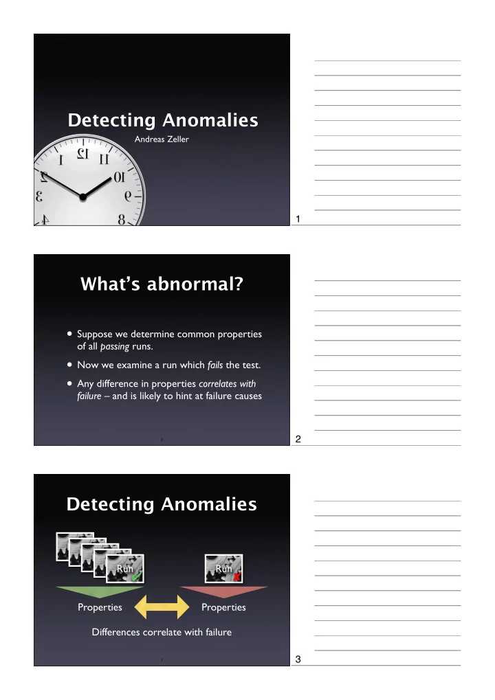
• Suppose we determine common properties
• f all passing runs.
• Now we examine a run which fails the test.
• Any difference in properties correlates with

failure – and is likely to hint at failure causes

2

Detecting Anomalies

3

Run Run Run Run Run Run

✔ ✘

Properties Properties Differences correlate with failure

1 2 3

Properties

4

Data properties that hold in all runs:

• “At f(), x is odd”
• “0 ≤ x ≤ 10 during the run”

Code properties that hold in all runs:

• “f() is always executed”
• “After open(), we eventually have close()”

Techniques

5

Dynamic Invariants Value Ranges Sampled Values

Techniques

6

Dynamic Invariants Value Ranges Sampled Values

4 5 6

Dynamic Invariants

7

Run Run Run Run Run Run

✔ ✘

At f(), x is odd At f(), x = 2 Invariant Property

Daikon

8

• Determines invariants from program runs
• Written by Michael Ernst et al. (1998–)
• C++, Java, Lisp, and other languages
• analyzed up to 13,000 lines of code

public int ex1511(int[] b, int n) { int s = 0; int i = 0; while (i != n) { s = s + b[i]; i = i + 1; } return s; }

Postcondition

b[] = orig(b[]) return == sum(b)

Precondition

n == size(b[]) b != null n <= 13 n >= 7

Daikon

9

• Run with 100 randomly generated arrays
• f length 7–13

7 8 9

Daikon

10

Run Run Run Run Run Trace Invariant Invariant Invariant Invariant

✔

get trace filter invariants report results

Postcondition

b[] = orig(b[]) return == sum(b)

Getting the Trace

11

Run Run Run Run Run Trace

✔

• Records all variable values at all function

entries and exits

• Uses VALGRIND to create the trace

Filtering Invariants

12

Trace Invariant Invariant Invariant Invariant

• Daikon has a library of

invariant patterns over variables and constants

• Only matching patterns are

preserved

10 11 12

Method Specifications

13

x = 6 x ∈ {2, 5, –30} x < y y = 5x + 10 z = 4x +12y +3 z = fn(x, y) A subseq B x ∈ A sorted(A)

using primitive data using composite data checked at method entry + exit

Object Invariants

14

string.content[string.length] = ‘\0’ node.left.value ≤ node.right.value this.next.last = this checked at entry + exit of public methods

Matching Invariants

15

A == B s size(b[]) n

public int ex1511(int[] b, int n) { int s = 0; int i = 0; while (i != n) { s = s + b[i]; i = i + 1; } return s; }

sum(b[]) return

• rig(n)

Pattern Variables …

13 14 15

== s n size( b[]) sum (b[])

• rig(

n) ret s n size(b[]) sum(b[])

• rig(n)

ret

Matching Invariants

16

s i n A == B s size(b[]) n sum(b[]) return

• rig(n)

Pattern Variables …

run 1

✘ ✘ ✘ ✘ ✘ ✘ ✘ ✘ ✘ ✘

== s n size( b[]) sum (b[])

• rig(

n) ret s n size(b[]) sum(b[])

• rig(n)

ret

Matching Invariants

17

s i n A == B s size(b[]) n sum(b[]) return

• rig(n)

Pattern Variables … ✘ ✘ ✘ ✘ ✘ ✘ ✘ ✘ ✘ ✘

run 2

✘ ✘ ✘ ✘ ✘ ✘ ✘ ✘ ✘ ✘

== s n size( b[]) sum (b[])

• rig(

n) ret s n size(b[]) sum(b[])

• rig(n)

ret

Matching Invariants

18

s i n A == B s size(b[]) n sum(b[]) return

• rig(n)

Pattern Variables … ✘ ✘ ✘ ✘ ✘ ✘ ✘ ✘ ✘ ✘

run 3

✘ ✘ ✘ ✘ ✘ ✘ ✘ ✘ ✘ ✘

16 17 18

== s n size( b[]) sum (b[])

• rig(

n) ret s n size(b[]) sum(b[])

• rig(n)

ret

Matching Invariants

19

s == sum(b[]) ✘ ✘ ✘ ✘ ✘ ✘ ✘ ✘ ✘ ✘ ✘ ✘ ✘ ✘ ✘ ✘ ✘ ✘ ✘ ✘ s == ret n == size(b[]) ret == sum(b[])

Matching Invariants

20

s == sum(b[]) s == ret n == size(b[]) ret == sum(b[])

public int ex1511(int[] b, int n) { int s = 0; int i = 0; while (i != n) { s = s + b[i]; i = i + 1; } return s; }

Enhancing Relevance

• Handle polymorphic variables
• Check for derived values
• Eliminate redundant invariants
• Set statistical threshold for relevance
• Verify correctness with static analysis

21

19 20 polymorphic variables: treat “object x” like “int x” if possible derived values: have “size(…)” as extra value to compare against redundant invariants: like x > 0 => x >= 0 statistical threshold: to eliminate random occurrences verify correctness: to make sure invariants always hold 21

Daikon Discussed

• As long as some property can be observed,

it can be added as a pattern

• Pattern vocabulary determines the

invariants that can be found (“sum()”, etc.)

• Checking all patterns (and combinations!)

is expensive

• Trivial invariants must be eliminated

22

Techniques

23

Dynamic Invariants Value Ranges Sampled Values

Dynamic Invariants

24

Run Run Run Run Run Run

✔ ✘

At f(), x is odd At f(), x = 2 Invariant Property Can we check this

• n the fly?

22 23 24

Diduce

25

• Determines invariants and violations
• Written by Sudheendra Hangal and Monica

Lam (2001)

• Java bytecode
• analyzed > 30,000 lines of code

Diduce

26

Run Run Run Run Run Run

✔ ✘

Invariant Property Training mode Checking mode

Training Mode

27

Run Run Run Run Run

✔

Invariant

• Start with empty set
• f invariants
• Adjust invariants

according to values found during run

25 26 27

Invariants in Diduce

For each variable, Diduce has a pair (V, M)

• V = initial value of variable
• M = range of values: i-th bit of M is cleared

if value change in i-th bit was observed

• With each assignment of a new value W,

M is updated to M := M ∧ ¬ (W ⊗ V)

• Differences are stored in same format

28

Training Example

29

Code i Values Differences Invariant

i = 10

1010 1010 1111 – –

i = 10

i += 1

1011 1010 1110 1 1111 10 ≤ i ≤ 11 ∧ |i′ – i| = 1

i += 1

1100 1010 1000 1 1111

8 ≤ i ≤ 15 ∧ |i′ – i| = 1

i += 1

1101 1010 1000 1 1111

8 ≤ i ≤ 15 ∧ |i′ – i| = 1

i += 2

1111 1010 1000 1 1101 8 ≤ i ≤ 15 ∧ |i′ – i| ≤ 2

V M V M

During checking, clearing an M-bit is an anomaly

30

• Less space and time requirements
• Invariants are computed on the fly
• Smaller set of invariants
• Less precise invariants

Diduce vs. Daikon

28 In Code, i = 10 is decimal 10; i, V, M are binary values. 29 30

Techniques

31

Dynamic Invariants Value Ranges Sampled Values

Detecting Anomalies

32

Run Run Run Run Run Run

✔ ✘

Properties Properties Differences correlate with failure How do we collect data in the field?

Liblit’s Sampling

33

• We want properties of runs in the field
• Collecting all this data is too expensive
• Would a sample suffice?
• Sampling experiment by Liblit et al. (2003)

31 32 33

Return Values

• Hypothesis: function return values correlate

with failure or success

• Classified into positive / zero / negative

34

CCRYPT fails

• CCRYPT is an interactive encryption tool
• When CCRYPT asks user for information

before overwriting a file, and user responds with EOF, CCRYPT crashes

• 3,000 random runs
• Of 1,170 predicates, only file_exists() > 0

and xreadline() == 0 correlate with failure

35

Liblit’s Sampling

36

Run Run Run Run Run

✔

Properties

• Can we apply this

technique to remote runs, too?

• 1 out of 1000 return

values was sampled

• Performance loss <4%

34 35 36

500 1000 1500 2000 2500 3000 20 40 60 80 100 120 140

Number of successful trials used Number of "good" features left

Failure Correlation

37

After 3,000 runs,

• nly five predicates are left

that correlate with failure

Web Services

38

• Sampling is first choice for web services
• Have 1 out of 100 users run an

instrumented version of the web service

• Correlate instrumentation data with failure
• After sufficient number of runs, we can

automatically identify the anomaly

Techniques

39

Dynamic Invariants Value Ranges Sampled Values

37 38 39

Anomalies and Causes

40

• An anomaly is not a cause, but a correlation
• Although correlation ≠ causation,

anomalies can be excellent hints

• Future belongs to those who exploit
• Correlations in multiple runs
• Causation in experiments

41

Concepts

Comparing data abstractions shows anomalies correlated with failure Variety of abstractions and implementations Anomalies can be excellent hints Future: Integration of anomalies + causes

42 This work is licensed under the Creative Commons Attribution License. To view a copy of this license, visit http://creativecommons.org/licenses/by/1.0

• r send a letter to Creative Commons, 559 Abbott Way, Stanford, California 94305, USA.

40 41 42