Mendelian randomization: From genetic association to epidemiological - - PowerPoint PPT Presentation

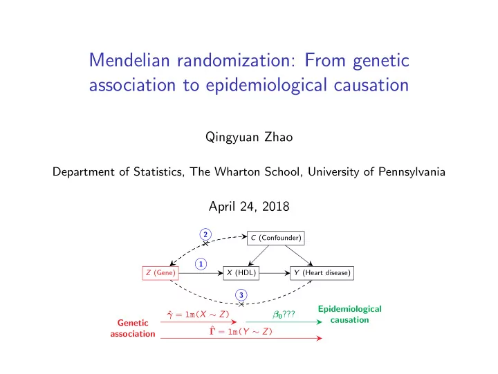
Mendelian randomization: From genetic association to epidemiological causation

Qingyuan Zhao

Department of Statistics, The Wharton School, University of Pennsylvania

April 24, 2018

Z (Gene) X (HDL) Y (Heart disease) C (Confounder) 1 2

×

3

×

ˆ γ = lm(X ∼ Z) ˆ Γ = lm(Y ∼ Z) β0??? Genetic association Epidemiological causation

1/33

Motivation: Epidemiology of cardiovascular diseases

◮ Cardiovascular diseases take the lives of 17.7 million people every

year, 31% of all global deaths.1

◮ Risk factors: hypertension, high cholesterol, smoking, . . . ◮ Ascertainment of a risk factor requires a large body of studies.

Expert opinions, case reports, animal studies Observational studies (case-control and cohort design) Natural experiments (Mendelian randomization) RCTs Quality of evidence

This talk

Figure: (A rough) Hierarchy of evidence.2

1Source: World Health Organization www.who.int/cardiovascular_diseases/en/ 2Based on: American Academy of Pediatrics clinical guidelines. Gidding, et al. (2012). “Developing the 2011 Integrated Pediatric Guidelines for Cardiovascular Risk Reduction.” Pediatrics 129(5).

2/33

The Lipid Hypothesis

“Decreasing blood cholesterol significantly reduces the risk of cardiovascular diseases.”3

1913 First evidence from a rabbit study. 1950s – 1980s Accumulation of evidence from observational studies. Transformation to the LDL hypothesis. 1970s Discoveries of the regulation of LDL cholesterol → Brown and Goldstein winning the Nobel prize in 1985. 1980s More evidence from US Coronary Primary Prevention Trial. 1990s Skepticism continue until landmark statin trials. 2010s Reaffirmation from Mendelian randomization.

However, the role of HDL cholesterol remains quite controversial.

3History based on: Academy of Medical Sciences Working Group (2007). “Identifying the environmental causes of disease: how should we decide what to believe and when to take action?” Academy of Medical Sciences.

3/33

The HDL Hypothesis

“HDL is protective against heart diseases.”4

1960s Formulation of the hypothesis from observational studies. The inverse association has been firmly established over the years. 1980s Supporting evidence from animal studies. But... 2000s Null findings from studies of Mendelian disorders. 2010s Failed RCTs, though each has its own caveats. 2010s Null findings from Mendelian randomization. “I’d say the HDL hypothesis is on the ropes right now,” said

• Dr. James A. de Lemos . . . Dr. Kathiresan said. “I tell them, ’ It

means you are at increased risk, but I don’t know if raising it will affect your risk.”’ — New York Times, May 16, 2012.

◮ Reasons of null findings: flawed design, lack of power, HDL function

hypothesis . . .

◮ We will reassess the evidence for HDL using a new design and

new statistical methods of Mendelian randomization.

4History based on: Rader and Hovingh (2014). “HDL and cardiovascular disease” Lancet 384.

4/33

Fundamental challenge of observational studies

“Correlation is not causation”. Observational studies = Enumerating confounders

◮ Idea: Conditioning on possible sources of spurious correlation. ◮ For HDL and heart disease, confounders include:

◮ Age. ◮ Sex. ◮ Smoking status. ◮ Diabetes. ◮ Blood pressure. ◮ . . .

◮ Fundamental challenge: We can never be sure this list is

complete.

◮ The promise of Mendelian randomization: unbiased estimation of

causal effect without enumerating confounders.

5/33

What is Mendelian randomization (MR)?

“Using genetic variants as instrumental variables.” Causal diagram for instrumental variables (IV)

Z (Gene) X (HDL) Y (Heart disease) C (Confounder) 1 2

×

3

× Core IV assumptions

• 1. Relevance: Z is associated with the exposure (X).
• 2. Effective random assignment: Z is independent of the

unmeasured confounder (C).

• 3. Exclusion restriction: Z cannot have any direct effect on the
• utcome (Y ).

6/33

Examine the core IV assumptions for MR

Z (Gene) X (HDL) Y (Heart disease) C (Confounder) 1 2

×

3

×

Criterion 1

• Massive pool of potential IVs,

Large-scale GWAS identifies many causal variants Criterion 2

• Due to Mendel’s Second Law

Criterion 3 ? Problematic because of wide-spread pleiotropy (multiple functions of genes).

Additional challenges

◮ Many genetic variants are only weakly associated with X. ◮ Most GWAS data come in summary-statistics format due to privacy.

7/33

MR studies in epidemiology

Surging interest in MR5

100 200 300 400 2005 2010 2015

Year Publication count ◮ MR methods are also increasingly used in human genetics.6

Conventional design: a 2012 MR study of HDL in Lancet7

Methods . . . First, we used as an instrument a single nucleotide polymorphism (SNP) in the endothelial lipase gene (LIPG Asn396Ser) . . . Second, we used as an instrument a genetic score consisting of 14 common SNPs that exclusively associate with HDL cholesterol . . .

5Thomson Reuters Web of Science, topic “Mendelian randomization”, www.webofknowledge.com. 6Gamazon, E. et al. (2015). “A gene-based association method for mapping traits using reference transcriptome data.” Nature Genetics 47. 7Example from: Voight et al. (2012). “Plasma HDL cholesterol and risk of myocardial infarction: a mendelian randomisation study.” Lancet 380: 572–580.

8/33

New methods for MR

Part 1: Increased robustness to pleiotropy

We will derive an estimator that is robust to both

• 1. Sparse pleiotropy/invalid IV.

◮ Works of Hyunseung Kang and coauthors.8

• 2. Dense but balanced pleiotropy.

◮ Works of Jack Bowden, Stephen Burgess and coauthors (e.g.

MR-Egger).9

Part 2: Increased efficiency in genome-wide MR

◮ Due to “missing heritability”, we would like to use as many SNPs as

possible to gain statistical power.

◮ Example: for height, there are extremely large number of causal

variants tiny effect sizes, spreading widely across the genome.10

◮ Statistical insights are needed to guarantee increased efficiency.

8Kang, H. et al. (2016). “Instrumental variables estimation with some invalid instruments and its application to Mendelian randomization.” Journal of American Statistical Association, 111. 9Bowden, J. et al. (2015). “Mendelian randomization with invalid instruments: effect estimation and bias detection through Egger regression.” International Journal of Epidemiology, 44. 10Shi, H. et al. (2016). “Contrasting the genetic architecture of 30 complex traits from summary association data.” American Journal of Human Genetics, 99. See also a 2017 Cell paper by Boyle et al.

9/33

Rest of the talk

Part 0: Data Structure & Modeling Assumptions Part 1: Increased robustness to pleiotropy Part 2: Increased efficiency in genome-wide MR

10/33

Outline

Part 0: Data Structure & Modeling Assumptions Part 1: Increased robustness to pleiotropy Evolution of pleiotropy models: Assumption 2.1 → 2.2 → 2.3 Evolution of statistical methods: PS → APS → RAPS Example: BMI and blood pressure Part 2: Increased efficiency in genome-wide MR RAPS with Empirical Partially Bayes Example: HDL and Coronary Heart Disease

11/33

Working example

Instrumental variables Z1:p: Single nucleotide polymorphisms (SNPs). Exposure variable X: Body mass index (BMI). Outcome variable Y : Systolic blood pressure (SBP).

Data preprocessing for two-sample summary-data MR

Dataset BMI-FEM BMI-MAL SBP-UKBB Source GIANT (female) GIANT (male) UK BioBank Sample size 171977 152893 317754 GWAS lm(X ∼ Zj) lm(X ∼ Zj) lm(Y ∼ Zj) Coefficient Used for selection ˆ γj ˆ Γj

• Std. Err.

σXj σYj Step 1 Use BMI-FEM to select significant (p-value ≤ 5 × 10−8) and independent SNPs (p = 25). Step 2 Use BMI-MAL to obtain (ˆ γj, σXj), j = 1 : p. Step 3 Use SBP-UKBB to obtain (ˆ Γj, σYj), j = 1 : p.

12/33

Assumption 1

Measurement error model

ˆ γ ˆ Γ

• ∼ N
• γ

Γ

• ,
• ΣX

ΣY

• ,

ΣX = diag(σ2

X1, . . . , σ2 Xp),

ΣY = diag(σ2

Y 1, . . . , σ2 Yp).

Pre-processing warrants Assumption 1

Dataset BMI-FEM BMI-MAL SBP-UKBB GWAS lm(X ∼ Zj) lm(X ∼ Zj) lm(Y ∼ Zj) Coefficient Used for selection ˆ γj ˆ Γj

• Std. Err.

σXj σYj

◮ Large sample size ⇒ CLT. ◮ Independence due to

• 1. Non-overlapping samples (in all three datasets).
• 2. Independent SNPs.

13/33

Assumption 2

Linking the genetic associations

The causal effect β0 satisfies Γ ≈ β0γ. This contains two claims:

• 1. The relationship is approximately linear.
• 2. The slope β0 has a causal interpretation.

Heuristic: Linear structural equation model

Assume all the IVs are valid. X =

p

• j=1

γjZj + ηXC + EX, Y = β0X +

p

• j=1

αjZj + ηY C + EY =

p

• j=1

(β0γj

• Γj

)Zj +

p

• j=1

αjZj

• 0 by exclusion restriction

+ f (C, EX, EY )

• independent of Z

14/33

Statistical problem

Genetic association

inference

= ⇒ Epidemiological causation (ˆ γj, ˆ Γj, σXj, σYj)j=1:p = ⇒ β0

Z (Gene) X (HDL) Y (Heart disease) C (Confounder) 1 2

×

3

×

ˆ γ = lm(X ∼ Z) ˆ Γ = lm(Y ∼ Z) β0??? Genetic association Epidemiological causation

15/33

Outline

Part 0: Data Structure & Modeling Assumptions Part 1: Increased robustness to pleiotropy Evolution of pleiotropy models: Assumption 2.1 → 2.2 → 2.3 Evolution of statistical methods: PS → APS → RAPS Example: BMI and blood pressure Part 2: Increased efficiency in genome-wide MR RAPS with Empirical Partially Bayes Example: HDL and Coronary Heart Disease

16/33

Assumptions 1 & 2.1 = ⇒ Profile score (PS)

Asumption 2.1: No pleiotropy

The linear relation Γj = β0γj is true for every j = 1, . . . , p.

◮ Log-likelihood of the data (up to additive constant):

l(β, γ1, . . . , γp) = −1 2

• p
• j=1

(ˆ γj − γj)2 σ2

Xj

+

p

• j=1

(ˆ Γj − γjβ)2 σ2

Yj

• .

◮ Profile likelihood: l(β) = max γ

l(β, γ) = −1 2

p

• j=1

(ˆ Γj − βˆ γj)2 σ2

Yj + β2σ2 Xj

.

◮ The MLE solves the profile score (PS) equation l′(ˆ

βPS) = 0.

◮ This estimator is an extension of the limited information

maximum likelihood (LIML) of Anderson and Rubin (1949)11 to the two-sample summary-data setting.

◮ Consistency and asymptotic normality can be proven.

11Anderson, T. , & Rubin, H. (1949). “Estimation of the parameters of a single equation in a complete system of stochastic equations.” Annals of Mathematical Statistics, 20.

17/33

Diagnostic plots show clear overdispersion

BMI-SBP Example (continued)

◮ Left (p = 25, psel < 5 · 10−8): Scatter-plot of GWAS summary data. ◮ Right (p = 160, psel < 10−4): Q-Q plot of standardized residual

ˆ tj = ˆ Γj − ˆ βˆ γj

• ˆ

β2σ2

Xj + σ2 Yj

.

• −0.05

0.00 0.05 0.000 0.025 0.050 0.075

SNP effect on BMI SNP effect on SBP

rs11191593 −5 5 10 −3 −2 −1 1 2 3

Quantile of standard normal Standardized residual

18/33

Why Assumption 2.1 failed?

Answer: pleiotropy (direct effect on the outcome).

Heuristic: Linear structural equation model (with invalid IVs)

X =

p

• j=1

γjZj + ηXC + EX, Y = β0X +

p

• j=1

αjZj + ηY C + EY =

p

• j=1

(β0γj + αj

• Γj

)Zj + f (C, EX, EY )

• independent of Z

Assumption 2.2: Random independent pleiotropy

Assume αj = Γj − β0γj is independent of γj and αj

i.i.d.

∼ N(0, τ 2

0 ).

19/33

Assumption 2.2 is consistent with genetic theory

This ubiquitous pleiotropy model is consistent (or not inconsistent) with the current understanding of genetic effects:

◮ Fisher’s infinitesimal model (1918). ◮ Leading edge perspective on pleiotropy12

“In summary, the omnigenic model of complex disease proposes that essentially any gene with regulatory variants in at least one tissue that contributes to disease pathogenesis is likely to have nontrivial effects on risk for that disease. Furthermore, the relative effect sizes are such that, since core genes are hugely outnumbered by peripheral genes, a large fraction of the total genetic contribution to disease comes from peripheral genes that do not play direct roles in disease.”

12Boyle, E. et al. (2017). “An expanded view of complex traits: from polygenic to omnigenic”. Cell 169, p1177–1186

20/33

Back to statistics: Failure of the profile likelihood

◮ The profile likelihood under Assumption 2.2 is given by

l(β, τ 2) = −1 2

p

• j=1

(ˆ Γj − βˆ γj)2 (σ2

Yj + τ 2) + β2σ2 Xj

+ log(σ2

Yj + τ 2), ◮ Easy to verify

E ∂ ∂β l(β0, τ 2

0 )

• = 0.

◮ But the other score function is biased:

∂ ∂τ 2 l(β, τ 2) = 1 2

p

• j=1

(ˆ Γj − βˆ γj)2

• (σ2

Yj + τ 2) + β2σ2 Xj

2 − 1 σ2

Yj + τ 2 . ◮ This is not too surprising as we are profiling out p nuisance

parameters γ1, · · · , γp (the Neyman-Scott problem).

21/33

Assumptions 1 & 2.2 = ⇒ Adjusted profile score (APS)

◮ We take the approach of McCullagh & Tibshirani (1990)13 to

modify the profile score ψ1(β, τ 2) = − ∂ ∂β l(β, τ 2), ψ2(β, τ 2) =

p

• j=1

σ2

Xj

• (ˆ

Γj − βˆ γj)2

• (σ2

Yj + τ 2) + β2σ2 Xj

2 − 1 (σ2

Yj + τ 2) + β2σ2 Xj

• .

◮ Trivial roots: β → ±∞ or τ 2 → ∞. ◮ Let ˆ

βAPS be the non-trivial finite solution.

Theorem

Let Assumptions 1 & 2.2 be given and assume σ2 = O(1/n) and (β0, pτ 2

0 ) is in

a bounded set B. If p → ∞ and p/n2 → 0, then

• 1. With probability going to 1 there exists a solution in B.
• 2. All solutions in B are consistent: ˆ

βAPS

p

→ β0 and pˆ τ 2

APS − pτ 2 p

→ 0.

◮ Can obtain asymptotic normality assuming p/n → λ ∈ (0, ∞).

13McCullagh, P. & Tibshirani, R. (1990). “A simple method for the adjustment of profile likelihoods”. Journal of the Royal Statistical Society. Series B (Methodological), 52.

22/33

Diagnostic plots show influential outlier

◮ Same 160 SNPs (psel < 10−4).

Left: Q-Q plot of std. residuals; Right: Influence of a single SNP.

rs11191593 −2.5 0.0 2.5 5.0 −3 −2 −1 1 2 3

Quantile of standard normal Standardized residual

rs11191593 0.24 0.28 0.32 0.36 2 5 10 20 50 100 200

Instrument strength (F−statistic) Leave−one−out estimate ◮ A clear outlier: rs11191593, with high influence (right plot). ◮ A GWAS catalog search reveals that this SNP is strongly associated with

reticulocyte (immature red blood cell) count.14

◮ Slightly underdispersed (probably because β is underestimated).

14Astle, W. et al. (2016). “The allelic landscape of human blood cell trait variation and links to common complex disease.” Cell 167: 1415-1429.

23/33

Assumptions 1 & 2.3 = ⇒ RAPS

Assumption 2.3: Random pleiotropy with outliers

Most αj ∼ N(0, τ 2

0 ), but some |αj| might be very large.

Robust adjusted profile score (RAPS)

◮ Define standardized residual: tj(β, τ 2) =

ˆ Γj − βˆ γj

• (σ2

Yj + τ 2) + β2σ2 Xj

.

◮ For some robust loss function ρ, the RAPS are

ψ(ρ)

1 (β, τ 2) = p

• j=1

ρ′(tj) · ∂ ∂β tj, ψ(ρ)

2 (β, τ 2) = p

• j=1

σ2

Xj

tj · ρ′(tj) − E[Tρ′(T)] (σ2

Yj + τ 2) + β2σ2 Xj

, for T ∼ N(0, 1).

◮ Reduces to APS when ρ(t) = t2/2. ◮ General theory is quite difficult, but local identifiability can be prove. ◮ Asymptotic normality can be established assuming consistency and

additional technical conditions.

24/33

Diagnostic plots show satisfactory fit

◮ Same 160 SNPs, now using RAPS with Huber’s loss function.

rs11191593 −3 3 6 −3 −2 −1 1 2 3

Quantile of standard normal Standardized residual

rs11191593 0.35 0.37 0.39 0.41 2 5 10 20 50 100 200

Instrument strength (F−statistic) Leave−one−out estimate ◮ Influence of the outlier rs11191593 is limited. ◮ Can further reduce its influence using redescending score (e.g.

Tukey’s biweight).

25/33

Comparison of the methods

In the BMI-SBP example

◮ MR-Egger: Weighted least squares of ˆ

Γj against ˆ γj (ignoring measurement error in ˆ γj and weak IV bias). MR-Egger ˆ β = 0.51 (SE 0.10) Profile score (PS) ˆ β = 0.61 (SE 0.05) Adjusted PS (APS) ˆ β = 0.30 (SE 0.16) Robust APS (RAPS) w. Huber ˆ β = 0.38 (SE 0.12)

In a simulation study

• ●
• ●
• ●
• ●
• Assumption 2.1

Assumption 2.2 Assumption 2.3 0.0 0.5 1.0 0.0 0.5 1.0 0.0 0.5 1.0 RAPS APS PS Egger

β ^

26/33

Outline

Part 0: Data Structure & Modeling Assumptions Part 1: Increased robustness to pleiotropy Evolution of pleiotropy models: Assumption 2.1 → 2.2 → 2.3 Evolution of statistical methods: PS → APS → RAPS Example: BMI and blood pressure Part 2: Increased efficiency in genome-wide MR RAPS with Empirical Partially Bayes Example: HDL and Coronary Heart Disease

27/33

Towards genome-wide MR

Unsatisfactory property of profile score (PS)

◮ Using Taylor’s expansion we can show Var(ˆ

βPS) ≈ V1/V 2

2 , where

V1 =

p

• j=1

γ2

j σ2 Yj + Γ2 j σ2 Xj + σ2 Xjσ2 Yj

(σ2

Yj + β2 0σ2 Xj)2

, V2 =

p

• j=1

γ2

j σ2 Yj + Γ2 j σ2 Xj

(σ2

Yj + β2 0σ2 Xj)2 . ◮ Paradoxical observation: adding a new SNP Zp+1 with γp+1 ≈ 0

increases the variance.

◮ This prohibits a truly “genome-wide” design of MR.

Semiparametric mixture model

◮ Why? Maximum likelihood is not efficient when p → ∞! ◮ Key idea: do not maximize the likelihood over γ, but over the

(empirical) distribution of γ.15

◮ However, the computation is intractable.

15Kiefer, J., & Wolfowitz, J. (1956). “Consistency of the maximum likelihood estimator in the presence of infinitely many incidental parameters”. Annals of Mathematical Statistics, 27, 887–906.

28/33

An alternative approach: Conditional score16

◮ Recall the log-likelihood of SNP j under Assumption 2.1 is

lj(β, γ) = −(ˆ γj − γj)2 2σ2

Xj

− (ˆ Γj − γjβ)2 2σ2

Yj

.

◮ Sufficient statistic for γj: ˆ

γj,MLE(β) = ˆ γj/σ2

Xj + βˆ

Γj/σ2

Yj

1/σ2

Xj + β2/σ2 Yj

.

◮ Conditional score is defined as

Cj(β) = ∂ ∂β lj(β, γ) − E ∂ ∂β lj(β, γ)

• ˆ

γj,MLE(β)

• = γj(ˆ

Γj − βˆ γj) σ2

Yj + β2σ2 Xj

.

◮ Observation 1: γj only appears as weight to “residual” ˆ

Γj − βˆ γj.

◮ Observation 2: ˆ

γj,MLE(β) is independent of ˆ Γj − βˆ γj.

◮ A general class of unbiased estimating equations:

p

• j=1

f (ˆ γj,MLE(β)) · (ˆ Γj − βˆ γj) σ2

Yj + β2σ2 Xj

= 0

◮ Reduces to MLE/profile score if f is identity.

16This method is based on Lindsay, B. (1985). “Using empirical partially Bayes inference for increased efficiency”. Annals of Statistics, 13, 914–931.

29/33

Empirical partially Bayes

◮ Lindsay showed that the optimal choice is the Bayes estimate of γj

f (ˆ γj,MLE) = E[γj|ˆ γj,MLE(β)].

◮ Since the distribution of γ is unknown, he suggested to use

empirical Bayes.

◮ The entire approach is partially Bayes because only the nuisance

parameters γ are modeled in a Bayesian way.

Implementation to genome-wide MR

◮ It is more convenient to model the effect sizes γj/σXj. ◮ We find that a good prior is the spike-and-slab Gaussian mixture. ◮ Selective shrinkage is important to increase efficiency. ◮ The whole approach can be extended to Assumptions 2.2 & 2.3 to

account for pleiotropy.

30/33

Application to HDL and coronary heart disease

Dataset

◮ Used a 2010 GWAS of blood lipids to select 1122 independent SNPs

not associated with LDL or triglycerides (p-value ≥ 0.01).

◮ 23 SNPs were genome-wide significant for HDL. ◮ HDL dataset: an non-overlapping 2013 GWAS of blood lipids. ◮ Coronary artery disease dataset: CARDIoGRAMplusC4D consortium.

Fitted prior for γj/σXj

◮ Spike: p1 = 0.91, σ1 = 0.73; ◮ Slab: p2 = 0.09, σ2 = 4.57.

Increase of efficiency (rough estimates from simulation)

Conventional MR

↑100%

= ⇒ Genome-wide MR

↑20%

= ⇒ Empirical partially Bayes.

31/33

Visualization of empirical partially Bayes

MLE Shrinkage 5 10 −2 2 −2 2

Absolute weight Standardized residual

23 genome-wide significant SNPs in the selection GWAS.

• Rest 1099 SNPs.

32/33

Results

◮ Method: RAPS with Huber’s loss + empirical partially Bayes. ◮ Scale: Odds ratio (95% CI) per 1 SD increase of LDL/HDL.

LDL HDL

Observational study

2009 JAMA 1.50 (1.39–1.61) 0.78 (0.74–0.82)

Previous MR

2012 Lancet 2.13 (1.69–2.69) 0.93 (0.68–1.26) 2016 JAMA Cardiology 1.68 (1.51–1.87) 0.95 (0.85–1.06)

New MR

Significant SNPs 1.76 (1.53–2.03) 0.88 (0.74–1.04) All SNPs 1.61 (1.45–1.80) 0.82 (0.73–0.91)

Caveats and future work

◮ It is unclear if the selected SNPs are truly unrelated to LDL or

triglycerides = ⇒ Our pleiotropy model might be insufficient.

◮ Estimates using strong instruments and weak instruments are not identical

= ⇒ The causal mechanism might be heterogeneous.

◮ The CARDIoGRAMplusC4D seems to have a small fraction of overlapping

samples = ⇒ We are working on a correction.

Conclusion

It is perhaps too soon to give up hope on the HDL hypothesis.

33/33

Acknowledgment

Collaborators

Jingshu Wang (Penn), Dylan Small (Penn), Jack Bowden (Bristol), Gibran Hemani (Bristol), Yang Chen (Michigan).

References

◮ Statistical inference in two-sample Mendelian randomization using

robust adjusted profile score. arXiv: 1801.09652.

◮ A genome-wide design and an empirical partially Bayes approach to

increase the power of Mendelian randomization, with application to the effect of blood lipids on cardiovascular disease. arXiv: 1804.07371.

Software

◮ R package mr.raps is available on CRAN. ◮ Can be directly called from the TwoSampleMR platform

(https://github.com/MRCIEU/TwoSampleMR).