Marija Vucelja Gregory Falkovich Konstantin S. Turitsyn Courant - - PowerPoint PPT Presentation

Fractal contours of scalar in a 2D smooth random flow

Courant Institute of Mathematical Sciences, Weizmann Institute of Sciences, MIT

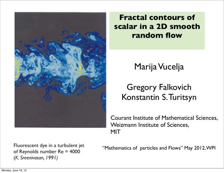
Fluorescent dye in a turbulent jet

• f Reynolds number Re = 4000

(K. Sreenivasan, 1991)

Marija Vucelja

Gregory Falkovich Konstantin S. Turitsyn

“Mathematics of particles and Flows” May 2012, WPI

Monday, June 18, 12

Mixing and transport

• The basic understanding of turbulent mixing and transport:

Taylor, Richardson, Kolmogorov, Obukhov and Corrsin...

from dimensional arguments: the average rate of spreading or mixing of e.g. a smoke plume.

• The statistics of the large fluctuations is a more

difficult problem.The practical relevance:

• the probability of a pollutant concentration exceeding some

tolerable level as it spreads from a source.

• the role of large concentration fluctuations in controlling the rate
• f slow (high order) chemical reactions (e.g. in the process of

atmospheric ozone destruction).

Monday, June 18, 12

Zero modes

multipoint correlation functions of scalar and gradient:

Schraiman, Siggia, Chertkov, Falkovich, Kolokolov, Lebedev, Gawedzki, Bernard, Kupiainen (1994-2000)

dθ dt = ∂θ ∂t + (v · r)θ = ϕ

1 2 3

Geometry of points that started close by...

˙ R(t) = v(R(t), t)

hθ(r1, t) . . . θ(rN, t)i = Z t

1

hϕ(R(t0

1), t0 1). . . ϕ(R(t0 1), t0 N)i dt0

• 1. . . dt0

N

θ(R(t), t) = Z t

1

ϕ(R(t0), t0) dt0

Monday, June 18, 12

Passive scalar evolution

We studied a passive scalar under the action of pumping, diffusion, advection in smooth 2D flow with Lagrangian chaos. ϕ(t, r)

∂tθ(t, r) + (v(t, r) · r)θ(t, r) = κdr2θ(t, r) + ϕ(t, r)

pumping diffusion

κd

molecular diffusion coefficient pumping scale

L

Poisson process of independently adding size-L blobs of passive scalar at random positions and with random amplitudes

Monday, June 18, 12

Smooth 2d flow field

Batchelor regime Batchelor 1959 Kraichnan model Kraichnan 1968 The velocity field: random, smooth and incompressible white in time and of spatially linear velocity profile hσij(t)σkl(t0)i=λ[3δikδjlδijδklδilδjk]δ(t t0) tensor of the local (Lagrangian) velocity gradients σij = ∂vi ∂rj λ Lyapunov exponent

Monday, June 18, 12

Batchelor regime

v(t, R1(t)) − v(R2(t)) = σ(t, R2(t))(R1(t) − R2(t))

Spatial scales

⌘ ≡ (⌫3/✏)1/4

kinematic viscosity Kolmogorov (viscous) scale valid when

|R1(t) − R2(t)| < η

pumping scale

ν

✏ energy dissipation

L

diffusion scale Prandtl number

rd ≡ p κd/λ Pr ⌘ ν/κd 1

Monday, June 18, 12

rd L L2 rd

Velocity Forcing Scalar blob evolution

Monday, June 18, 12

Smooth flows - a simplest example of mixing

• large-scale mixing in the Earth atmosphere where the

turbulence spectrum (the velocity gradients are then well-defined and the flow can be locally considered smooth).

• flows in the phase space of dynamical systems.

Mixing in smooth flows is provided by exponential separation of trajectories and Lagrangian chaos. We consider an incompressible fluid flows which correspond to Hamiltonian flows in phase space.

k−3

Monday, June 18, 12

NEW computational method

• exploiting the linearity of the reaction diffusion

equation

• method of characteristic to solve for a single

spherical blob of scalar

θ(t0, r0) = Θ0 exp[−(r0 − rc)2/(2L2)]

θ(t, r0) = Θ0L2 p det I(t, t0) e− 1

2 (r(t)−rc)I−1(t,t0)(r(t)−rc)

at a later time initial form of blob

r(t) ≡ W(t)r(t0)

defines evolution operator W(t)

I(t, t0) ≡

• WW T

(t) + κd Z t dt0W(t)W(t0)1[W(t)W 1(t0)]T

moment of inertia

Monday, June 18, 12

seven values specify a blob at time t:

Semi-analytic method allows HUGE resolutions

I11, I12, I21, Θ0, rc, t0

Summing over the blobs can get passive scalar field. Large enough number of blobs assures the Gaussianity of pumping statistics. Conventional methods out used are pseudospectral and thus always one is limited by the slow decay (logarithmic) of the passive scalar pair correlation function.

θ(t, r0) = Θ0L2 p det I(t, t0) e− 1

2 (r(t)−rc)I−1(t,t0)(r(t)−rc)

Monday, June 18, 12

top: 2400 L x 360 L (L pumping scale) bottom: zoomed inset

A long iso-contour

Monday, June 18, 12

v ϕ v ϕ v

fjords l λ1

L

Appearance of fjords of isolines of scalar

creation of fjords

snapshot scalar field 75 L x 75 L

IMPORTANT: diffusion randomly reconnects the curves

Monday, June 18, 12

Statistics of nodal lines

Expectations - “trivial statistics”

• pumping alone would produce a Gaussian field whose zero isolines

are smooth at the scales below L, while at larger scales they are equivalent to critical percolation ( ).

• does not change the statistics of as it just rearranges it; the flow

stretches isolines uniformly at the direction of and contracts them transversal to it.

SLE6 , D0 = 7/4 θ θ v λ1

Non-trivial statistics and its isolines arises from an interplay of velocity, pumping and finite diffusivity or finite resolution, which leads to the dissipation of scalar and reconnection of isolines that came closer than the resolution scale.

Actually: Non-trivial statistics

Monday, June 18, 12

Non-gaussian field

substituting PDF in FP equation first term

Indeed we know that correlation functions include cumulants. Our scalar is a non-gaussian field...

Monday, June 18, 12

No conformal invariance

F4 = f ✓r12r34 r13r24 , r12r34 r14r23 ◆ (r12r34r14r23r13r24)a

Balkovsky et al 1995

Conformal symmetry restricts a four point correlation function:

F4 = F(r12, r34) + F(r13, r24) + F(r14, r23)

For passive scalar we know that

F4 = hθ1θ2θ3θ4i

four point correlation function

F(x, y) = (xy)a/2 + (xy−2)a/2 + (x−2y)a/2 F4 = (r12r34)2a + (r13r24)2a + (r14r23)2a

BOTH equations satisfied by i.e. to a Gaussian statistics, which is not the case, as we have just

• shown. Passive scalar is not in any way close to a free field and its

statistics is not conformally invariant.

NOTE: this is not Wick theorem!

Monday, June 18, 12

PDF of contour perimeters

10 10

2

10

4

10

−4

10

−2

P/L P[log(P/L)]

/ = 0.05 / = 0.02 / = 0.01 / = 0.005 rd/L = 0.06 rd/L = 0.03 rd/L = 0.015 (1.04±0.02) 3/2

3/2 (1.04±0.02)

P - perimeter

ν/λ rd/L

pumping frequency resolution

All collapse on top of one another (lower three curves shifted down by dividing by 10)

Monday, June 18, 12

PDF of sizes (mean radius R)

10

−2

10 10

2

0.0001 0.001 0.01 0.1

R/L P[log(R/L)]

/ = 0.05 / = 0.02 / = 0.01 / = 0.005 rd/L = 0.06 rd/L = 0.03 rd/L = 0.015 3/2 3/2

R ⌘ p h(ρ hρi)2i

All collapse on top of one another (lower three curves shifted down by dividing by 10)

Monday, June 18, 12

Salient features of PDFs of P and R

10

−2

10 10

2

0.0001 0.001 0.01 0.1

R/L P[log(R/L)]

/ = 0.05 / = 0.02 / = 0.01 / = 0.005 rd/L = 0.06 rd/L = 0.03 rd/L = 0.015 3/2 3/2

10 10

2

10

4

10

−4

10

−2

P/L P[log(P/L)]

/ = 0.05 / = 0.02 / = 0.01 / = 0.005 rd/L = 0.06 rd/L = 0.03 rd/L = 0.015 (1.04±0.02) 3/2

3/2 (1.04±0.02)

Left tails: 3/2. Contours shorter than L must appear when pumping cuts a piece off a thin long contour, the probability of such a cut is . Extra factor in the PDF may appear because to be observed small contours need to survive without being swallowed by further pumping events. Since creation and survival are independent events, their probabilities are multiplied.

P ∝ R √ P ∝ √ R

Right tail PDF of P: In log coordinates the tail is close to P −1

P(P) ∝ P −2

(no theoretical explanation so far)

Monday, June 18, 12

1e+03 1e+04 1e+05 1e+06 1e+07 0.1 1 10 100

[i pq

i()]1/(1-q)

/L

q = 0 q = 2 q = 4 1 1.6 1.5 1.6 1.7 1.8 0 1 2 3 4

Dq q

Dq ≡ lim

ε→0 log

@

N(ε)

X

i

pq

i (ε)

1 A [(q − 1) log(ε)]−1

generalized box counting fractal dimension fractal dimension is scale dependent

1.55 ÷ 1.7 1.0

Monday, June 18, 12

1 1.2 1.4 1.6 1 10 100

D0 /L

1.0

1.55 ÷ 1.7

box counting fractal dimension estimated from It is scale dependent: bellow forcing scale it is smooth, above it is fractal.

d log N(ε)/ d log(L/ε)

box counting fractal dimension

D0 = lim

✏→0

ln(N(✏)) ln(✏−1)

Monday, June 18, 12

Mono fractals

Monday, June 18, 12

Characterize curves with SLE (Schramm-Loewner Evolution)

dgt(z) dt = 2 gt(z) − at

• conformal map with which the tip of the curve is

mapped into the real axis

• driving function
• for Markovian successive maps the driving function at is

a standard Brownian motion (Schramm, 2000):

Loewner, 1923 Schramm, 2000

at gt at = √κBt

Monday, June 18, 12

2000 4000 6000 8000 10000 0.2 0.4 0.6 0.8 t [L2] <2>/t

N1= 486, T = 100, rd/L = 0.06 N2= 451, T = 100, rd/L = 0.03 N3= 363, T = 100, rd/L = 0.015 N4= 175, T = 50, rd/L = 0.06 N5= 88, T = 20, rd/L = 0.06

number of contours we averaged over

depends on the evolution time, does not depend on the

resolution

The curves of different resolutions are of different length since the time of

the Loewner map is measured in the units of length squared and for a better resolution we used a smaller physical window.

Ni κ

single velocity realization

Monday, June 18, 12

0.2 0.4 0.6 0.8 1 2000 4000 6000 8000 10000 <2>/t t [L2] N1 = 154 N2 = 237 N3 = 351

10 20 100 200 300

<2>/t t [L2] n1 = 62 n3 = 151

Effective diffusivity for different velocity realizations (x, y) → ⇣ x, rd L y ⌘

inset

Monday, June 18, 12

Surprises

Statistics of bending of long isolines

• If there was only pumping then the scalar would be a short-

correlated field on scales r > L (such as percolation).

• Without diffusion and with infinite resolution, velocity only

distorts the field. The distorted field is not SLE (Kennedy, 2008),

still the driving functions tells us a lot about the geometrical properties of bending.

SLE in experiments: While the restoration procedure itself may be not very practical since real flows consist of many such domains oriented randomly, the very possibility of it means potential availability of very useful exact formulae describing the statistics of contours.

Monday, June 18, 12

• ur simulations our runs

Summarizing

• The distribution of contours over sizes and perimeters is

shown to depend neither on the flow realization nor on the resolution (diffusion) scale

• The scalar isolines are found fractal/smooth at the scales

larger/smaller than the pumping scale.

• Driving function of the Loewner map: Behaves

like diffusion with diffusivity independent of the resolution yet, most surprisingly, dependent on the velocity realization and the time - beyond the time on which the statistics of the scalar is stabilized:

λ−1 ln ✓ L rd ◆ rd

Tsλ ≤ 4 Tsλ ∈ {20, 50, 100}

Monday, June 18, 12

Future ideas

• explain velocity realization dependence of diffusivity
• investigate in detail non-stationarity for isolines?
• other simple models in stochastic geometry

Monday, June 18, 12