MA/CSSE 473 Day 36 Kruskal proof recap Prim Data Structures and - PDF document

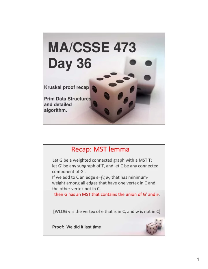
MA/CSSE 473 Day 36 Kruskal proof recap Prim Data Structures and detailed algorithm. Recap: MST lemma Let G be a weighted connected graph with a MST T; let G ′ be any subgraph of T, and let C be any connected component of G ′ . If we add to C an edge e=(v,w) that has minimum ‐ weight among all edges that have one vertex in C and the other vertex not in C, then G has an MST that contains the union of G ′ and e . [WLOG v is the vertex of e that is in C, and w is not in C] Proof: We did it last time 1

Recall Kruskal’s algorithm • To find a MST: • Start with a graph containing all of G’s n vertices and none of its edges. • for i = 1 to n – 1: – Among all of G’s edges that can be added without creating a cycle, add one that has minimal weight. Does this algorithm produce an MST for G? Does Kruskal produce a MST? • Claim: After every step of Kruskal’s algorithm, we have a set of edges that is part of an MST Work on the quiz questions • Base case … with one or two other students • Induction step: – Induction Assumption: before adding an edge we have a subgraph of an MST – We must show that after adding the next edge we have a subgraph of an MST – Suppose that the most recently added edge is e = (v, w). – Let C be the component (of the “before adding e” MST subgraph) that contains v • Note that there must be such a component and that it is unique. – Are all of the conditions of MST lemma met? – Thus the new graph is a subgraph of an MST of G 2

Does Prim produce an MST? • Proof similar to Kruskal. • It's done in the textbook Recap: Prim’s Algorithm for Minimal Spanning Tree • Start with T as a single vertex of G (which is a MST for a single ‐ node graph). • for i = 1 to n – 1: – Among all edges of G that connect a vertex in T to a vertex that is not yet in T, add to T a minimum ‐ weight edge. At each stage, T is a MST for a connected subgraph of G. A simple idea; but how to do it efficiently? Many ideas in my presentation are from Johnsonbaugh, Algorithms , 2004, Pearson/Prentice Hall 3

Main Data Structure for Prim • Start with adjacency ‐ list representation of G • Let V be all of the vertices of G, and let V T the subset consisting of the vertices that we have placed in the tree so far • We need a way to keep track of "fringe vertices" – i.e. edges that have one vertex in V T and the other vertex in V – V T • Fringe vertices need to be ordered by edge weight – E.g., in a priority queue • What is the most efficient way to implement a priority queue? Prim detailed algorithm step 1 • Create an indirect minheap from the adjacency ‐ list representation of G – Each heap entry contains a vertex and its weight – The vertices in the heap are those not yet in T – Weight associated with each vertex v is the minimum weight of an edge that connects v to some vertex in T – If there is no such edge, v's weight is infinite • Initially all vertices except start are in heap, have infinite weight – Vertices in the heap whose weights are not infinite are the fringe vertices – Fringe vertices are candidates to be the next vertex (with its associated edge) added to the tree 4

Prim detailed algorithm step 2 • Loop: – Delete min weight vertex w from heap, add it to T – We may then be able to decrease the weights associated with one or more vertices that are adjacent to w Indirect minheap overview • We need an operation that a standard binary heap doesn't support: decrease(vertex, newWeight) – Decreases the value associated with a heap element – We also want to quickly find an element in the heap • Instead of putting vertices and associated edge weights directly in the heap: – Put them in an array called key[] – Put references to these keys in the heap 5

Indirect Min Heap methods operation description run time init(key) build a MinHeap from the array of keys Ѳ (n) del() delete and return the (location in key[ ] of Ѳ (log n) the) minimum element isIn(w) is vertex w currently in the heap? Ѳ (1) keyVal(w) The weight associated with vertex w Ѳ (1) (minimum weight of an edge from that vertex to some adjacent vertex that is in the tree). decrease(w, changes the weight associated with vertex w Ѳ (log n) newWeight) to newWeight (which must be smaller than w's current weight) Indirect MinHeap Representation Draw the tree diagram of the heap • outof[i] tells us which key is in location i in the heap • into[j] tells us where in the heap key[j] resides • into[outof[i]] = i, and outof[into[j]] = j. • To swap the 15 and 63 (not that we'd want to do this): temp = outof[2] outof[2] = outof[4] outof[4] = temp temp = into[outof[2]] into[outof[2]] = into[outof[4]] into[outof[4]] = temp 6

MinHeap class, part 1 MinHeap class, part 2 7

MinHeap class, part 3 MinHeap class, part 4 8

Prim Algorithm AdjacencyListGraph class 9

MinHeap implementation • An indirect heap. We keep the keys in place in an array, and use another array, "outof", to hold the positions of these keys within the heap. • To make lookup faster, another array, "into" tells where to find an element in the heap. • i = into[j] iff j = out of[i] • Picture shows it for a maxHeap, but the idea is the same: MinHeap code part 1 We will not discuss the details in class; the code is mainly here so we can look at it and see that the running times for the various methods are as advertised 10

MinHeap code part 2 NOTE: delete could be simpler, but I kept pointers to the deleted nodes around, to make it easy to implement heapsort later. N calls to delete() leave the outof array in indirect reverse sorted order. MinHeap code part 3 11

Preview: Data Structures for Kruskal • A sorted list of edges (edge list, not adjacency list) • Disjoint subsets of vertices, representing the connected components at each stage. – Start with n subsets, each containing one vertex. – End with one subset containing all vertices. • Disjoint Set ADT has 3 operations: – makeset(i) : creates a singleton set containing i. – findset(i): returns a "canonical" member of its subset. • I.e., if i and j are elements of the same subset, findset(i) == findset(j) – union(i, j): merges the subsets containing i and j into a single subset. Q37 ‐ 1 Example of operations • makeset (1) • union(4, 6) • makeset (2) • union (1,3) • makeset (3) • union(4, 5) • makeset (4) • findset(2) • makeset (5) • findset(5) • makeset (6) What are the sets after these operations? 12

Kruskal Algorithm What can we Assume vertices are numbered 1...n say about (n = |V|) efficiency of Sort edge list by weight (increasing order) this algorithm for i = 1..n: makeset(i) (in terms of |V| i, count, tree = 1, 0, [] and |E|)? while count < n-1: if findset(edgelist[i].v) != findset(edgelist[i].w): tree += [edgelist[i]] count += 1 union(edgelist[i].v, edgelist[i].w) i += 1 return tree Set Representation • Each disjoint set is a tree, with the "marked" element as its root • Efficient representation of the trees: – an array called parent – parent[i] contains the index of i’s parent. – If i is a root, parent[i]=i 5 1 7 4 2 3 6 8 13

Using this representation • makeset(i): • findset(i): • mergetrees(i,j): – assume that i and j are the marked elements from different sets. • union(i,j): – assume that i and j are elements from different sets Analysis • Assume that we are going to do n makeset operations followed by m union/find operations • time for makeset? • worst case time for findset? • worst case time for union? • Worst case for all m union/find operations? • worst case for total? • What if m < n? • Write the formula to use min 14

Can we keep the trees from growing so fast? • Make the shorter tree the child of the taller one • What do we need to add to the representation? • rewrite makeset, mergetrees • findset & union are unchanged. • What can we say about the maximum height of a k ‐ node tree? Q37 ‐ 5 Theorem: max height of a k ‐ node tree T produced by these algorithms is  lg k  • Base case… • Induction hypothesis… • Induction step: – Let T be a k ‐ node tree – T is the union of two trees: T 1 with k 1 nodes and height h 1 T 2 with k 2 nodes and height h 2 – What can we say about the heights of these trees? – Case 1: h 1 ≠ h 2 . Height of T is – Case 2: h 1 =h 2 . WLOG Assume k 1 ≥ k 2 . Then k 2 ≤ k/2. Height of tree is 1 + h2 ≤ … Q37 ‐ 5 15

Worst ‐ case running time • Again, assume n makeset operations, followed by m union/find operations. • If m > n • If m < n Speed it up a little more • Path compression: Whenever we do a findset operation, change the parent pointer of each node that we pass through on the way to the root so that it now points directly to the root. • Replace the height array by a rank array, since it now is only an upper bound for the height. • Look at makeset, findset, mergetrees (on next slides) 16

Makeset This algorithm represents the set { i } as a one ‐ node tree and initializes its rank to 0. def makeset3 ( i ): parent [ i ] = i rank [ i ] = 0 Findset • This algorithm returns the root of the tree to which i belongs and makes every node on the path from i to the root (except the root itself) a child of the root. def findset (i): root = i while root != parent [ root ]: root = parent [ root ] j = parent [ i ] while j != root : parent [ i ] = root i = j j = parent [ i ] return root 17