m c ( s ) end . s p I.N. & P .O. Spring 2006 I.N. & P - PowerPoint PPT Presentation

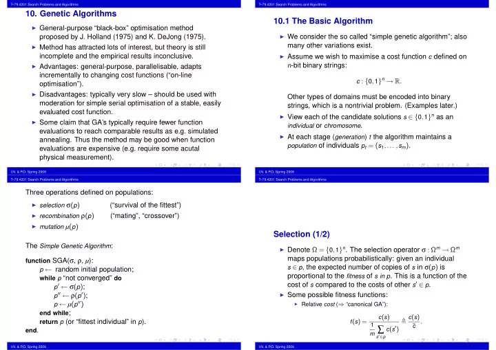
T–79.4201 Search Problems and Algorithms T–79.4201 Search Problems and Algorithms 10. Genetic Algorithms 10.1 The Basic Algorithm ◮ General-purpose “black-box” optimisation method ◮ We consider the so called “simple genetic algorithm”; also proposed by J. Holland (1975) and K. DeJong (1975). many other variations exist. ◮ Method has attracted lots of interest, but theory is still ◮ Assume we wish to maximise a cost function c defined on incomplete and the empirical results inconclusive. ◮ Advantages: general-purpose, parallelisable, adapts n -bit binary strings: incrementally to changing cost functions (“on-line c : { 0 , 1 } n → R . optimisation”). ◮ Disadvantages: typically very slow – should be used with Other types of domains must be encoded into binary moderation for simple serial optimisation of a stable, easily strings, which is a nontrivial problem. (Examples later.) evaluated cost function. ◮ View each of the candidate solutions s ∈ { 0 , 1 } n as an ◮ Some claim that GA’s typically require fewer function individual or chromosome . evaluations to reach comparable results as e.g. simulated ◮ At each stage ( generation ) t the algorithm maintains a annealing. Thus the method may be good when function population of individuals p t = ( s 1 ,... , s m ) . evaluations are expensive (e.g. require some acutal physical measurement). I.N. & P .O. Spring 2006 I.N. & P .O. Spring 2006 T–79.4201 Search Problems and Algorithms T–79.4201 Search Problems and Algorithms Three operations defined on populations: ◮ selection σ ( p ) (“survival of the fittest”) ◮ recombination ρ ( p ) (“mating”, “crossover”) ◮ mutation µ ( p ) Selection (1/2) The Simple Genetic Algorithm : ◮ Denote Ω = { 0 , 1 } n . The selection operator σ : Ω m → Ω m maps populations probabilistically: given an individual function SGA( σ , ρ , µ ): s ∈ p , the expected number of copies of s in σ ( p ) is p ← random initial population; proportional to the fitness of s in p . This is a function of the while p “not converged” do cost of s compared to the costs of other s ′ ∈ p . p ′ ← σ ( p ) ; p ′′ ← ρ ( p ′ ) ; ◮ Some possible fitness functions: p ← µ ( p ′′ ) ◮ Relative cost ( ⇒ “canonical GA”): end while ; c ( s ) � c ( s ) return p (or “fittest individual” in p ). f ( s ) = c . 1 ¯ m ∑ c ( s ′ ) end . s ′ ∈ p I.N. & P .O. Spring 2006 I.N. & P .O. Spring 2006

T–79.4201 Search Problems and Algorithms T–79.4201 Search Problems and Algorithms ◮ Relative rank : Selection (2/2) r ( s ) 2 Once the fitness of individuals has been evaluated, selection f ( s ) = = m + 1 · r ( s ) , 1 m ∑ r ( s ′ ) can be performed in different ways: s ′ ∈ p ◮ Roulette-wheel selection (“stochastic sampling with where r ( s ) is the rank of individual s in a worst-to-best ordering of replacement”): all s ′ ∈ p . ◮ Assign to each individual s ∈ p a probability to be selected in proportion to its fitness value f ( s ) . Select m individuals according to this distribution. ◮ Pictorially: Divide a roulette wheel into m sectors of width proportional to f ( s 1 ) ,... , f ( s m ) . Spin the wheel m times. ◮ Remainder stochastic sampling : ◮ For each s ∈ p , select deterministically as many copies of s as indicated by the integer part of f ( s ) . After this, perform stochastic sampling on the fractional parts of the f ( s ) . ◮ Pictorially: Divide a fixed disk into m sectors of width proportional to f ( s 1 ) ,... , f ( s m ) . Place an outer wheel around the disk, with m equally-spaced pointers. Spin the outer wheel once. I.N. & P .O. Spring 2006 I.N. & P .O. Spring 2006 T–79.4201 Search Problems and Algorithms T–79.4201 Search Problems and Algorithms Recombination (2/2) Recombination (1/2) Possible crossover operators: ◮ Given a population p , choose two random individuals ◮ 1-point crossover: s , s ′ ∈ p . With probablity p ρ , apply a crossover operator 1 1 0 1 0 0 1 1 0 0 1 0 1 1 0 0 0 1 1 0 0 1 ρ ( s , s ′ ) to produce two new offspring individuals t , t ′ that 0 1 1 0 1 0 1 1 0 1 1 1 1 0 1 1 0 1 1 0 1 1 replace s , s ′ in the population. ◮ 2-point crossover: ◮ Repeat the crossover throughout the population. Denote 1 1 0 1 0 0 1 1 0 0 1 1 1 1 0 1 0 1 1 0 0 1 the total effect on the population as p ′ = ρ ( p ) . 0 11 0 1 0 1 1 0 1 1 0 1 0 1 0 0 1 1 0 1 1 p ρ ◮ Practical implementation: choose 2 · m random pairs from p and apply crossover deterministically. ◮ uniform crossover: ◮ Typically p ρ ≈ 0 . 7 ... 0 . 9 . 1 1 0 1 0 0 1 1 0 0 1 0 1 0 1 1 0 1 1 0 0 1 0 1 1 0 1 0 1 1 0 1 1 1 1 0 1 1 0 1 1 0 0 1 I.N. & P .O. Spring 2006 I.N. & P .O. Spring 2006

T–79.4201 Search Problems and Algorithms T–79.4201 Search Problems and Algorithms 10.2 Analysis of GA’s Mutation Hyperplane sampling (1/4) ◮ Given population p , consider each bit of each individual ◮ A heuristic view of how a genetic algorithm works. and flip it with some small probability p µ . Denote the total ◮ A hyperplane (actually subcube) is a subset of Ω = { 0 , 1 } n , effect on the population as p ′ = µ ( p ) . where the values of some bits are fixed and other are free ◮ Typically, p µ ≈ 0 . 001 ... 0 . 01 . Apparently good choice: to vary. A hyperplane may be represented by a schema p µ = 1 / n for n -bit strings. H ∈ { 0 , 1 , ∗} n . ◮ Theoretically mutation is disruptive. Recombination and ◮ E.g. schema ’ 0 ∗ 1 ∗∗ ’ represents the 3-dimensional selection should take care of optimisation; mutation is hyperplane (subcube) of { 0 , 1 } 5 where bit 1 is fixed to 0, bit needed only to (re)introduce “lost alleles”, alternative 3 is fixed to 1, and bits 2, 4, and 5 vary. values for bits that have the bits that have the same value ◮ Individual s ∈ { 0 , 1 } n samples hyperplane H , or matches the in all current individuals. corresponding schema if the fixed bits of H match the ◮ In practice mutation + selection = local search. Mutation, corresponding bits in s . (Denoted s ∈ H .) even with quite high values of p µ , can be efficient and is ◮ Note : given individual generally samples many hyperplanes often more important than recombination. simultaneously, e.g. individual ’ 101 ’ samples ’ 10 ∗ ’, ’ 1 ∗ 1 ’, etc. I.N. & P .O. Spring 2006 I.N. & P .O. Spring 2006 T–79.4201 Search Problems and Algorithms T–79.4201 Search Problems and Algorithms ◮ average fitness of hyperplane H in population p : 1 m ( H , p ) ∑ f ( H , p ) = f ( s , p ) s ∈ H ∩ p Hyperplane sampling (2/4) Define: Heuristic claim : selection drives the search towards hyperplanes ◮ order of hyperplane H : of higher average cost (quality). o ( H ) = number of fixed bits in H = n − dim H ◮ average cost of hyperplane H : 1 2 n − o ( H ) ∑ c ( H ) = c ( s ) s ∈ H ◮ m ( H , p ) = number of individuals in population p that sample hyperplane H . I.N. & P .O. Spring 2006 I.N. & P .O. Spring 2006

T–79.4201 Search Problems and Algorithms T–79.4201 Search Problems and Algorithms Here the current population of 21 individuals samples the hyperplanes so that e.g. ’ 000 ∗∗ ’ and ’ 010 ∗∗ ’ are sampled by three individual each, and ’ 100 ∗∗ ’ and ’ 101 ∗∗ ’ by two individual each. Hyperplane ’ 010 ∗∗ ’ has a rather low average fitness in this population, whereas ’ 111 ∗∗ ’ has a rather high average fitness. Hyperplane sampling (3/4) Consider e.g. the following cost function and partition of Ω into hyperplanes (in this case, intervals) of order 3: c(s) 000** 001** 010** 011** 100** 101** 110** 111** Ω I.N. & P .O. Spring 2006 I.N. & P .O. Spring 2006 T–79.4201 Search Problems and Algorithms T–79.4201 Search Problems and Algorithms Hyperplane sampling (3/4) The effect of crossover on schemata (1/2) Then the result of e.g. roulette wheel selection on this population might lead to elimination of some individuals and ◮ Consider a schema such as duplication of others: H = ∗∗ 11 ∗∗ 01 ∗ 1 ∗∗ � �� � c(s) ∆( H )= 7 and assume that it is represented in the current population by some s ∈ H . ◮ If s participates in a crossover operation and the crossover point is located between bit positions 3 and 10, then with large probability the offspring are no longer in H ( H is disrupted ). 000** 001** 010** 011** 100** 101** 110** 111** Ω ◮ On the other hand, if the crossover point is elsewhere, then Then, in terms of expected values, one can show that one of the offspring stays in H ( H is retained ). m ( H , σ ( p )) = m ( H , p ) · f ( H , p ) . I.N. & P .O. Spring 2006 I.N. & P .O. Spring 2006