LiNGAM combined with Instantaneous effects can be incorporated - - PDF document

2010/7/8 1

Non-Gaussian Methods for Learning Linear Structural Equation Models (Part II)

UAI 2010 Tutorial, Catalina Island

Shohei Shimizu and Yoshinobu Kawahara Osaka University

Equation Models (Part II)

Outline of Part II

Some recent advances in LiNGAM analysis:

• 1. LiNGAM combined with time-series models

– AR-LiNGAM (Hyvarinen et al., 2010) ARMA LiNGAM (Kawahara et al 2010) – ARMA-LiNGAM (Kawahara et al., 2010)

• 2. LiNGAM with latent confounders

– lvLiNGAM (Hoyer et al., 2006) – GroupLiNGAM (Kawahara et al, 2010)

LiNGAM combined with time-series models

Time-series analysis with LiNGAM

 How useful is it to analyze time-series data using

non-Gaussianity of data?

 Instantaneous effects can be incorporated explicitly

into account through LiNGAM analysis combined into account through LiNGAM analysis combined with classical time-series models:

– AR-LiNGAM (Hyvarinen et al.,2010) – ARMA-LiNGAM (Kawahara et al.,2010)

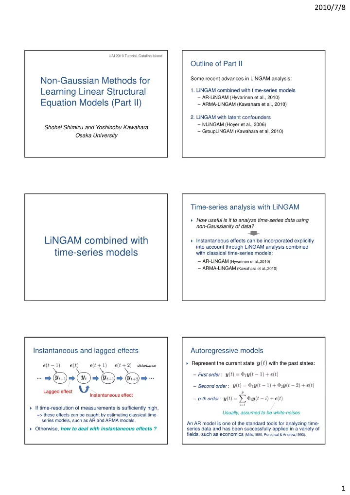
Instantaneous and lagged effects

Lagged effect

… …

disturbance

 If time-resolution of measurements is sufficiently high,

=> these effects can be caught by estimating classical time- series models, such as AR and ARMA models.

 Otherwise, how to deal with instantaneous effects ?

Instantaneous effect Lagged effect

Autoregressive models

 Represent the current state with the past states:

– First order : – Second order : – p-th order : Usually, assumed to be white-noises An AR model is one of the standard tools for analyzing time- series data and has been successfully applied in a variety of fields, such as economics (Mills,1990, Perceival & Andrew,1993).

2010/7/8 2

Incorporating instantaneous effects

 Introduce the instantaneous term into AR models

(AR-LiNGAM) (Hyvarinen et al.,2010): i = 1,…, p (AR-model) => i = 0, 1,…, p (AR-LiNGAM) How to estimate the model including instantaneous effects ? => 1. Assume that is non-Gaussian.

• 2. Apply LiNGAM analysis.

Estimation (1/2)

Relation between two models:

AR-model: AR-LiNGAM:

This is a SEM with non-Gaussian external influences.

Disturbance: Regression Coef.:

Estimation (2/2)

• 1. Estimate a multivariate AR model (i.e., ) and then

calculate .

• 2. Apply LiNGAM analysis to the estimated :

and calculate the matrix .

• 3. Using the estimated , calculate the parameters of

AR-LiNGAM through .

Extension to ARMA model (1/2)

 AR-model

– can estimate apparent effects or power-spectrum, – but cannot express direct relationships between variables in principle.

 ARMA (Autoregressive moving-average) model:

– More general representation for time-series data (exact representation of linear differential equations in discrete time-domain) (An AR-model is an asymptotic expansion of an ARMA-model.)

Extension to ARMA model (2/2)

The analogous relationships between ARMA models and ARMA-LiNGAM models still hold (Kawahara et al.,2010):

ARMA-model: ARMA-LiNGAM:

Again, this is a SEM with non-Gaussian external influences.

Disturbance: Regression Coef.:

Connection to Granger causality (1/2)

Granger causality* (Granger,1976, Boudjellaba,1992): The processes do not cause the process if and only if

Suppose a multivariate process is partitioned into ( ). The processes do not cause the process if and only if for all .

: Variance of prediction error of *) Granger causality is not necessarily a natural extension of the causality for i.i.d. data, which is usually defined based on the counter-factual model.

,

: Past sequence up to time t ,

2010/7/8 3

Connection to Granger causality (2/2)

• G. C.

ARMA model:

=>

(Boudjellaba,1992)

(Hyvarinen et al 2010 Kawahara et al 2010)

If the order in the sense of Granger causality completely agrees with the instantaneous effects, then the order is preserved even if the instantaneous effects are neglected.

ARMA-LiNGAM:

=>

+

(Hyvarinen et al.,2010, Kawahara et al.,2010)

Application to real data

Duplex-pendulum system:

Rad Analytic model for the duplex-pendulum system: Chaotic pattern Time[s]

Application to physical system (cont.)

Estimated lagged effects by AR- and ARMA-LiNGAM:

AR-LiNGAM ARMA-LiNGAM

Although dominant patterns are captured by both models, the chaotic effect is captured only by ARMA-LiNGAM.

t t-1 t t-2 t t-1 t t-2

Summary (LiNGAM combined with time-series models)

 Non-Gaussianity could be useful for analyzing time-series

data (AR-LiNGAM and ARMA-LiNGAM). – Instantaneous effects can be taken into account by using non-Gaussianity of disturbances.

 AR-LiNGAM (or ARMA-LiNGAM) is identified by first  AR-LiNGAM (or ARMA-LiNGAM) is identified by first

estimating a classical AR model (or ARMA-model) and then applying LiNGAM analysis on disturbance sequences.

 The order in the sense of Granger causality is satisfied if

and only if both of the instantaneous and lagged effects in AR-LiNGAM (or ARMA-LiNGAM) give the same order.

LiNGAM with Latent Confounders

Latent confounder

 Independent external influences (the assumption in LiNGAM)

=> No latent confounder (Spirtes et al., 2000)

Latent variable which is a parent of more than two observed variables

 A latent confounder induces dependency among external

influences:

Latent confounder

2010/7/8 4

Motivation of this topic

 Actual data might include latent confounders.

=> In the case, the assumption on LiNGAM that there is no latent confounders has been violated.

 How to overcome this ?

– IvLiNGAM (Hoyer et al.,06)

• Overcomplete ICA.

– GroupLiNGAM (Kawahara et al.,10)

• Extension of the principle of DirectLiNGAM to ‘set’.

Latent variable LiNGAM

 Introduce latent confounders f to LiNGAM model:

=> Overcomplete ICA

(Lewicki & Sejnowski 2000, Eriksson & Koivunen 2004)

How to classify f and e? and how to assign fi ?

non-Gaussian and independent

<=> A

Basic idea of lvLiNGAM

• 1. Remove external influences.
• 2. Find a pair of observed variables that has no
• bserved parents.

– Mark their common parent as a latent confounder. – The existence of such a pair is guaranteed by the The existence of such a pair is guaranteed by the assumption that “no latent confounder that has total effects to some observed variable and its descendants only.”

• 3. Repeat 1-2.

Find an external influence

The i-th row vector of A has non-zero at the j-th column and all zeros elsewhere:

Mixing matrix j-th col.

The j-th element of s is an external influence.

Find a latent confounder

• 1. If the j-th row vector ‘covers’ i-the row one:

=> is a parent of ( ).

ex.) non-zero element

is a parent of ( ).

• 2. If the i-th and j-th row vectors do not cover each other:

=> and have no order.

ex.)

If the i-th row vector ‘covers’ no other rows, has no observed parents.

Empirical example

Two different networks, which has the same ordering

• f variables, were estimated in this case.

Estimated network Original network

2010/7/8 5

Motivation of this topic

 Actual data might include latent confounders.

=> In the case, the assumption on LiNGAM that there is no latent confounders has been violated.

 How to overcome this ?

– IvLiNGAM (Hoyer et al.,06)

• Overcomplete ICA.

– GroupLiNGAM (Kawahara et al.,10)

• Extension of the principle of DirectLiNGAM to ‘set’.

Basic idea of GroupLiNGAM

 DirectLiNGAM

=> Variable ordering is estimated by iteratively finding an exogenous variable.

 GroupLiNGAM

p => Group ordering (i.e., ordering of sets of variables) is estimated by recursively finding an exogenous set (defined later). Applicable to data with latent confounders

Exogenous set

 Let the partition of variables be .

The subset of variables is said to be exogenous against , if the corresponding partition of the matrix B has the following form: . => Group ordering: {1,2} < {3}

ex.)

Exogenous set (cont.)

Lemma: a set of variables is exogenous if and only if is independent of its residual .

: Residual when is regressed on .

=> This lemma extends DirectLiNGAM to the ‘set’ case.

is independent of . is not independent of .

Identification of an exogenous set

Find a subset (U is the set of variables) s t Find a subset of variables that is independent of the residuals

Find an exogenous set =

Find a subset (U is the set of variables) s.t. where is a small real number. Some independence measure I, such as mutual information

(Kraskov et al.,2004) and HSIC (Gretton et al.,2005), is used.

Estimation (1/2)

Zero-one structure of matrix B still holds in SEMs of the exogenous set and the residuals, respectively. {1,2} < {3} < {4,5}

exogenous set residuals (S={1,2,3})

{1,2} {3} {4,5}

2010/7/8 6

Estimation (2/2)

Thus, the group ordering can be found by recursively finding a partition of variables into an exogenous set and the rest of the variables until no further partition is found.

{1 2 3 4 5} {1, 2, 3, 4, 5} {4, 5} {1, 2, 3} {3} {1, 2}

{1,2} < {3} < {4,5}

Associated graph

Application to sociology (1/2)

Father’s Education Father’s Son’s Education Son’s

Status attainment model based on domain knowledge*:

Father s Occupation Number of Sibilings

{1, 3, 6}<{5}<{4}<{2}

Son’s Occupation Son s Income

*) Dataset is obtained from sociological data repository, General Social Survey (www.norc.org/GSS+Website/)

Application to sociology (2/2)

Comparative results by ICA-LiNGAM, DirectLiNGAM and GroupLiNGAM ( is omitted because data is not well constructed): Domain knowledge: {1, 3, 6} < {5} < {4} (< {2}) ICA LiNGAM {5} {6} {3} {1} {4}

• ICA-LiNGAM: {5} < {6} < {3} < {1} < {4}
• DirectLiNGAM: {6} < {1} < {3} < {4} < {5}
• GroupLiNGAM: {6} < {1,3} < {5} < {4}

( and the mutual information is used as an independence measure.)

GroupLiNGAM seems to give a reasonable solution.

Summary (LiNGAM with Latent Confounders)

 Although LiNGAM analysis assume no latent confounder,

it is often violated in practice.

 We introduced two approaches that allow latent variables

in LiNGAM analysis.

– lvLiNGAM: (Overcomplete ICA) – lvLiNGAM: (Overcomplete ICA) – GroupLiNGAM: (Extension of DirectLiNGAM to ‘set’ case)

Summary

 We introduced some recent advances in LiNGAM analysis:

– LiNGAM combined with time-series models (AR-LiNGAM

(Hyvarinen et al., 2010), ARMA-LiNGAM (Kawahara et al.,2010))

– LiNGAM with latent variables (lvLiNGAM (Hoyer et al.,2006), GroupLiNGAM (Kawahara et al.,2010))

which is expected to make LiNGAM analysis be more applicable in practice.

 These are just small samples and there could exist several

new directions of future researche on LiNGAM analysis.