Lake Nutrient Classification Phosphorus Trophic State Lake Use - PDF document

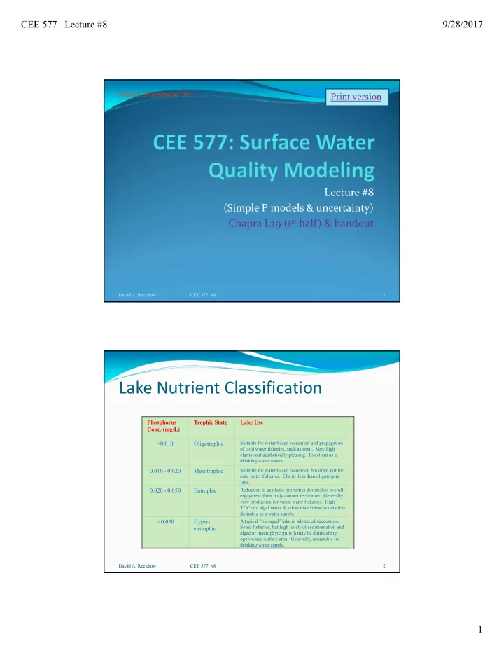
CEE 577 Lecture #8 9/28/2017 Updated: 28 September 2017 Print version Lecture #8 (Simple P models & uncertainty) Chapra L29 (1 st half) & handout David A. Reckhow CEE 577 #8 1 Lake Nutrient Classification Phosphorus Trophic State Lake Use Conc. (mg/L) Suitable for water-based recreation and propagation <0.010 Oligotrophic of cold water fisheries, such as trout. Very high clarity and aesthetically pleasing. Excellent as a drinking water source. 0.010 - 0.020 Mesotrophic Suitable for water-based recreation but often not for cold water fisheries. Clarity less than oligotrophic lake. 0.020 - 0.050 Eutrophic Reduction in aesthetic properties diminishes overall enjoyment from body contact recreation. Generally very productive for warm water fisheries. High TOC and algal tastes & odors make these waters less desirable as a water supply. > 0.050 Hyper- A typical "old-aged" lake in advanced succession. Some fisheries, but high levels of sedimentation and eutrophic algae or macrophyte growth may be diminishing open water surface area. Generally, unsuitable for drinking water supply. David A. Reckhow CEE 577 #8 2 1

CEE 577 Lecture #8 9/28/2017 Phosphorus and productivity David A. Reckhow CEE 577 #8 3 Clarity and productivity Chapra, pg 541 David A. Reckhow CEE 577 #8 4 2

CEE 577 Lecture #8 9/28/2017 Oxygen depletion and P David A. Reckhow CEE 577 #8 5 Empirical Modeling 10 A re a l P L o a d in g  Vollenweider’s (g /m 2 /y r) 1 phosphorus 0.1 loading plot Eutrophic 0.01  P=fn(L/Z) 1 10 100 1000 Mean Depth (m)  refer to Chapra, pg. 535 Oligotrophic Depth is H or Z David A. Reckhow CEE 577 #8 6 3

CEE 577 Lecture #8 9/28/2017 Total Maximum Daily Load (TMDL)  See lecture #38, extra topic  Definition (from DEP Website):  “A TMDL is the greatest amount of a pollutant that a waterbody can accept and still meet water quality standards for protecting public health and maintaining the designated beneficial uses of those waters for drinking, swimming, recreation, and fishing. A TMDL is implemented by specifying how much of that pollutant can come from point, nonpoint, and natural sources.”  “The TMDL provisions require states to identify and list waterbodies that are threatened or not meeting water quality standards despite controls on point source discharges.”  For MA studies see DEP website  http://www.mass.gov/eea/agencies/massdep/water/watershe ds/total ‐ maximum ‐ daily ‐ loads ‐ tmdls.html David A. Reckhow CEE 577 #8 7 Empirical P Models (cont.)  Vollenweider modifies earlier model for effects of flushing  x ‐ axis is equivalent to hydraulic overflow rate, L Q/A s . Z  David A. Reckhow CEE 577 #8 w 8 4

CEE 577 Lecture #8 9/28/2017 Simple Lake P Model  This model is based on a simple mass balance with terms for loading (W), settling, and outflow. There is no spatial, or temporal resolution dP    V W v PA QP s s dt  Dividing both sides by the surface area (A s ) gives: dP    H L v P q P s s dt  where, H is the lake depth, L is the areal loading (W/A s ) and q s is the overflow rate (Q/A s ). At steady state (dP/dt =0), the solution becomes: L  P  v q s s David A. Reckhow CEE 577 #8 9 Simple Lake P Model (cont.)  Based on data from 47 northern temperate lakes included in EPA's National Eutrophication Survey, the settling velocity (in m/yr) was found to be an empirical function of the overflow rate[1]:   11 . 6 0 . 2 v q s s  so substituting this into the steady state model above, we get: L  P  116 . 12 . q s [1] From: Reckhow, 1979 [JWPCF 51(8)2123-2128] “Uncertainty Analysis Applied to Vollenweider’s Phosphorus Loading Criterion” David A. Reckhow CEE 577 #8 10 5

CEE 577 Lecture #8 9/28/2017 Simple Lake P Model (cont.) L  P  116 . 12 . q s  where:  P = mean annual total phosphorus concentration (g ‐ P/m 3 or mg ‐ P/L)  L = mean annual areal phosphorus loading (g ‐ P/m 2 ‐ yr)  q s = mean annual areal water loading or overflow rate (m/yr) = Q/A s  This model was developed from lakes with the following characteristics  phosphorus concentrations in the range of 0.004 ‐ 0.135 mg/L  phosphorus loadings of 0.07 ‐ 31.4 g ‐ P/m 2 ‐ yr  overflow rates of 0.75 ‐ 187 m/yr.  It should not be used for lakes whose characteristics are outside of this range. David A. Reckhow CEE 577 #8 11 Simple Lake P Model (cont.)  When used properly, the log transform of the model has an estimated error (s mlog ) of 0.128. This value was determined from comparison of observed and predicted phosphorus concentrations in the 47 lakes. Therefore, considering error, the model can be written as:      log( )   P s 11 . 6 1 . 2 10 log L q m s David A. Reckhow CEE 577 #8 12 6

CEE 577 Lecture #8 9/28/2017 Modeling Perspectives From Chapra (pg 538) from: Reckhow, 1979 David A. Reckhow CEE 577 #8 13 Determination of Areal Water Loading (overflow rate)  q s = Q/A s  If Q is not directly measurable from inflow or outflow, then it can be estimated from:  Q = (A d x r) + (A s x Pr) where: q s = areal water loading (m/yr) Q = inflow water volume to lake (m 3 /yr) A d = watershed area (land surface) (m 2 ) A s = lake surface (m 2 ) r = total annual unit runoff (m/yr) Pr = mean annual net precipitation (m/yr) David A. Reckhow CEE 577 #8 14 7

CEE 577 Lecture #8 9/28/2017 Data Collection  Determine total drainage area (A d ) from a GIS database, or USGS maps, using a polar planimeter, or cut paper with squares.  Estimate the surface area of the lake (A s ). This may also be done by GIS or planimetry using a USGS map, or the cut paper method.  Estimate annual runoff (r) which is usually expressed in meters/year. This information is generally available from the USGS.  Determine average annual net precipitation (P r ), also expressed as meters/year. This information can usually be obtained from the USGS or the US Weather Service. David A. Reckhow CEE 577 #8 15 Determination of Areal Loading with Uncertainty  Total phosphorus mass loading (W) as proposed by Reckhow et al. (1980):  W = (Ec f x Area f ) + (Ec ag x Area ag ) + (Ec u x Area u ) + (Ec a x A s ) + (Ec st x #capita ‐ yrs x [1 ‐ S.R.]) + PSI where: Ec f = export coefficient for forest land (kg/ha-yr) Ec ag = export coefficient for agricultural land (kg/ha-yr) Ec u = export coefficient for urban area (kg/ha-yr) Ec a = export coefficient for atmospheric input (kg/ha-yr) Ec st = export coefficient to septic systems impacting the lake (kg/(capita-yr)-yr) Area f = area 1 of forested land (ha) Area ag = area of agricultural land (ha) Area u = area of urban land (ha) A s = surface area of lake (ha) #capita-yrs number of capita-years in watershed serviced by septic tank impacting the lake S.R. = soil retention coefficient (dimensionless) David A. Reckhow PSI = point source input (kg/yr) CEE 577 #8 16 8

CEE 577 Lecture #8 9/28/2017 Data Collection  Estimate land use drainage areas (forested, agricultural, urban).  This information may be available from:  local planning agencies  otherwise it may be obtained from GIS data.  For future projections, high and low estimates are needed for assessment of uncertainty  Choose Export Coefficients for each category.  Ranges should be selected for the major sources (often all but precipitation).  Choice depends on characteristics of watershed as compared to those previously studied, for which there already exists export coefficients. Other factors may play a role such as the use of phosphate detergents (will impact E cst ). David A. Reckhow CEE 577 #8 17 General P Export Coefficients  From Reckhow et al. 1980 Source Symbol Units High Mid-range Low Agricultural Ec ag kg/(ha-yr) 3.0 0.4-1.7 0.10 Forest Ec f kg/(ha-yr) 0.45 0.15-0.3 0.02 Precipitation Ec a kg/(ha-yr) 0.60 0.20-0.50 0.15 Urban Ec u kg/(ha-yr) 5.0 0.8-3.0 0.50 Input to septic tanks Ec st kg/(capita-yr) 1.8 0.4-0.9 0.3  Mattson & Isaac (1999)  Argue that MA may have a lower P export than the US average David A. Reckhow CEE 577 #8 18 9

CEE 577 Lecture #8 9/28/2017 Septic System Calculations  Estimate SR:  This is a number between 0 and 1 that indicates how well the soil and associated plants take up phosphorus. When it is low more of the phosphorus reaches the lake. Factors to consider include:  phosphorus adsorption capacity  natural drainage  permeability  slope  Estimate number of capita ‐ years on septic systems impacting lake  This requires some judgment, but usually a strip of about 20 ‐ 200 m wide surrounding the lake is considered the zone of influence. All septic systems within this zone would be counted in the following calculation: David A. Reckhow CEE 577 #8 19 Data Collection (cont.) Total # of = average # of X # days spent at X # of living units capita-years persons per unit per year within zone of living unit /360 influence  Estimate Point source inputs: possibly from NPDES permits  Now determine high, low and most likely estimates of W using above equation. These are obtained from high, low and most likely estimates of the various input parameters (note that the low value of S.R. should go with the high estimate of W, and vice versa). David A. Reckhow CEE 577 #8 20 10