Introduction to Deep Learning 1 / 24 Is it a question? Given - - PowerPoint PPT Presentation

Introduction to Deep Learning

1 / 24

Is it a question?

Given training data with categories A (◦) and B (×), say well drilling sites with different outcomes

2 / 24

Is it a question?

Given training data with categories A (◦) and B (×), say well drilling sites with different outcomes Question? How to classify the rest of points, say where should we propose a new drilling site for the desired outcome?

2 / 24

AI via Machine Learning

• 1. AI via Machine Learning has advanced radically over the past 10 year.

3 / 24

AI via Machine Learning

• 1. AI via Machine Learning has advanced radically over the past 10 year.
• 2. ML algorithms now achieve human-level performance or better on the

tasks such as

3 / 24

AI via Machine Learning

• 1. AI via Machine Learning has advanced radically over the past 10 year.
• 2. ML algorithms now achieve human-level performance or better on the

tasks such as

◮ face recognition ◮ optical character recognition ◮ speech recognition ◮ object recognition ◮ playing the game Go – in fact, defeated human champions 3 / 24

AI via Machine Learning

• 1. AI via Machine Learning has advanced radically over the past 10 year.
• 2. ML algorithms now achieve human-level performance or better on the

tasks such as

◮ face recognition ◮ optical character recognition ◮ speech recognition ◮ object recognition ◮ playing the game Go – in fact, defeated human champions

• 3. Deep Learning becomes the centerpiece of ML toolbox.

3 / 24

Deep Learning

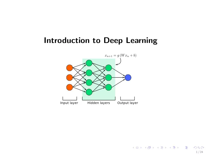
◮ Deep Learning = multilayered Artificial Neural Network (ANN).

4 / 24

Deep Learning

◮ Deep Learning = multilayered Artificial Neural Network (ANN). ◮ A simple ANN with four layers

Layer 1 (Input layer) Layer 2 Layer 3 Layer 4 (Output layer)

4 / 24

Deep Learning

◮ An ANN in a mathematically term

5 / 24

Deep Learning

◮ An ANN in a mathematically term

F(x) = σ

• W [4] σ
• W [3] σ(W [2]x + b[2]) + b[3]

+ b[4]

• 5 / 24

Deep Learning

◮ An ANN in a mathematically term

F(x) = σ

• W [4] σ
• W [3] σ(W [2]x + b[2]) + b[3]

+ b[4]

• where

◮ p := {(W [2], b[2]), (W [3], b[3]), (W [4], b[4])} are parameters to be

“trained/computed” from training data.

◮ σ(·) is an activiation function, say sigmoid function

σ(z) = 1 1 + e−z

5 / 24

Deep Learning

◮ The objective of training is to “minimize” a properly defined cost

function, say min

p Cost(p) ≡ 1

m

m

• i=1

F(x(i)) − y(i)2

2,

where {(x(i), y(i))} are training data

6 / 24

Deep Learning

◮ The objective of training is to “minimize” a properly defined cost

function, say min

p Cost(p) ≡ 1

m

m

• i=1

F(x(i)) − y(i)2

2,

where {(x(i), y(i))} are training data

◮ Steepest/gradient descent

p ← − p − τ ∇Cost(p) where τ is known as the learning rate.

6 / 24

Deep Learning

◮ The objective of training is to “minimize” a properly defined cost

function, say min

p Cost(p) ≡ 1

m

m

• i=1

F(x(i)) − y(i)2

2,

where {(x(i), y(i))} are training data

◮ Steepest/gradient descent

p ← − p − τ ∇Cost(p) where τ is known as the learning rate. The underlying operations of DL are stunningly simple, mostly matrix-vector products, but extremely intense.

6 / 24

Experiment 1

Given training data with categories A (◦) and B (×), say well drilling sites with different outcomes

7 / 24

Experiment 1

Given training data with categories A (◦) and B (×), say well drilling sites with different outcomes Question for DL: How to classify the rest of points, say where should we propose a new drilling site for the desired outcome?

7 / 24

Experiment 1

Classification after 90 seconds training on my desktop

8 / 24

Experiment 1

Classification after 90 seconds training on my desktop

8 / 24

Experiment 1

The value of Cost(W [·], b[·]):

9 / 24

Experiment 2

Given training data with categories A (◦) and B (×), say well drilling sites with different outcomes

10 / 24

Experiment 2

Given training data with categories A (◦) and B (×), say well drilling sites with different outcomes Question for DL: How to classify the rest of points, say where should we propose a new drilling site for the desired outcome?

10 / 24

Experiment 2

Classification after 90 seconds training on my desktop

11 / 24

Experiment 2

Classification after 90 seconds training on my desktop

11 / 24

Experiment 2

The value of Cost(W [·], b[·]):

12 / 24

Experiment 3

Given training data with categories A (◦) and B (×), say well drilling sites with different outcomes

13 / 24

Experiment 3

Given training data with categories A (◦) and B (×), say well drilling sites with different outcomes Question for DL: How to classify the rest of points, say where should we propose a new drilling site for the desired outcome?

13 / 24

Experiment 3

Classification after 16 seconds training on my desktop

14 / 24

Experiment 3

Classification after 16 seconds training on my desktop

14 / 24

Experiment 3

Classification after 38 seconds training on my desktop

15 / 24

Experiment 3

Classification after 38 seconds training on my desktop

15 / 24

Experiment 3

Classification after 46 seconds training on my desktop

16 / 24

Experiment 3

Classification after 46 seconds training on my desktop

16 / 24

Experiment 3

Classification after 62 seconds training on my desktop

17 / 24

Experiment 3

Classification after 62 seconds training on my desktop

17 / 24

Experiment 3

Classification after 83 seconds training on my desktop

18 / 24

Experiment 3

Classification after 83 seconds training on my desktop

18 / 24

Experiment 3

Classification after 156 seconds training on my desktop

19 / 24

Experiment 3

Classification after 156 seconds training on my desktop

19 / 24

Experiment 3

The value of Cost(W [·], b[·]): 16 38 46 62 83 156

20 / 24

Experiment 4

Given training data with categories A (◦) and B (×), say well drilling sites with different outcomes

21 / 24

Experiment 4

Given training data with categories A (◦) and B (×), say well drilling sites with different outcomes Question for DL: How to classify the rest of points, say where should we propose a new drilling site for the desired outcome?

21 / 24

Experiment 4

Classification after 90 seconds training on my desktop

22 / 24

Experiment 4

Classification after 90 seconds training on my desktop

22 / 24

Experiment 4

The value of Cost(W [·], b[·]):

23 / 24

“Perfect Storm”

• 1. The recent success of ANNs in ML, despite their long history, can be

contributed to a “perfect storm” of

24 / 24

“Perfect Storm”

• 1. The recent success of ANNs in ML, despite their long history, can be

contributed to a “perfect storm” of

◮ large labeled datasets; ◮ improved hardware; ◮ clever parameter constraints; ◮ advancements in optimization algorithms; ◮ more open sharing of stable, reliable code leveraging the latest in

methods.

24 / 24

“Perfect Storm”

• 1. The recent success of ANNs in ML, despite their long history, can be

contributed to a “perfect storm” of

◮ large labeled datasets; ◮ improved hardware; ◮ clever parameter constraints; ◮ advancements in optimization algorithms; ◮ more open sharing of stable, reliable code leveraging the latest in

methods.

• 2. ANN is simultaneously one of the simplest and most complex

methods:

24 / 24

“Perfect Storm”

• 1. The recent success of ANNs in ML, despite their long history, can be

contributed to a “perfect storm” of

◮ large labeled datasets; ◮ improved hardware; ◮ clever parameter constraints; ◮ advancements in optimization algorithms; ◮ more open sharing of stable, reliable code leveraging the latest in

methods.

• 2. ANN is simultaneously one of the simplest and most complex

methods:

◮ learning to model and parameterization ◮ capable of self-enhancement ◮ generic computation architecture ◮ executable on local HPC and on cloud ◮ broadly applicable but requires good understanding of the underlying

problems and algorthms

24 / 24